Bet Sizing With Skewed Returns

From The Logbook. The original article is reproduced in full, with minor grammar corrections; references to market conditions reflect the context in which it was written.

The continuous form of Kelly betting traditionally relies on the first two moments of the return distribution. This simplification does not consider the effects of higher-order moments like skewness and kurtosis. However, real-world stock returns often exhibit negative skew (a tendency for large losses) and positive excess kurtosis (a higher frequency of extreme returns), which significantly impact the distribution of outcomes. These characteristics imply that the standard Kelly formula underestimates the risks associated with large drawdowns and overstates the likelihood of achieving the expected growth rate. To more accurately optimize the growth rate, the formula should incorporate adjustments for skewness and kurtosis. By doing so, the strategy can better account for the asymmetry and fat tails present in actual return distributions, leading to a more robust and realistic measure of optimal leverage.

Review: Kelly Criterion

The Kelly Criterion is an approach to determine the optimal allocation of capital to maximize long-term growth of wealth. The core idea is to invest a proportion of capital that maximizes the logarithm of wealth, ensuring the highest expected geometric / compounded rate of growth over time (i.e. leads to higher wealth than any other strategy in the long run with probability 1) while avoiding the risk of ruin.

For a discrete outcome scenario, such as a gamble with known probabilities of winning and losing, the optimal betting fraction is

f^* = \frac{p}{b}- \frac{q}{a}

Where p is the probability of win, b is the factor by which wealth increases in the winning case, q is the probability of loss, and a is the factor by which wealth decreases in the losing case.

Continuous Kelly

For the continuous case of normally distributed return with known mean and variance, the optimal leverage factor to optimize the compounded rate of growth is

f^* = \frac{\mu}{\sigma^2}

We now show a proof sketch and in the process also determine how we can incorporate skewness and kurtosis into our estimate of the optimal leverage. Let our wealth at time n be represented as a product of bet fraction f and return on bet Xi

W_n = W_0 \prod_{i=1}^n (1+fX_i)

We take log-returns i.e. compounded rate of growth

\ln{\frac{W_n}{W_0}} = \sum_{i=1}^n \ln{(1+fX_i)}

The expectation of the above can be given by

\mathbb{E}[\ln{(W_n / W_0)}] = n\mathbb{E}[\ln{(1 + fX_n)}] = n \int{\ln(1+fx)g(x) \text{d}}x

where g(x) is the distribution of returns x. The optimal bet size f is clearly independent of n, so we can optimize the expectation with respect to f by taking the partial derivative with respect to f and setting the resulting term to 0. Before doing that, we can consider the Taylor approximation

\ln(1 + f x) = f x - \frac{1}{2} (f x)^2 + \frac{1}{3} (f x)^3 - \frac{1}{4} (f x)^4 + \dots

which transforms the target of optimization into

f \int x g(x) \, dx - \frac{1}{2} f^2 \int x^2 g(x) \, dx + \frac{1}{3} f^3 \int x^3 g(x) \, dx - \frac{1}{4} f^4 \int x^4 g(x) \, dx + \dots

defining moments of x under g

\mu = \int x g(x) \, dx, \quad \mu_2 = \int x^2 g(x) \, dx, \quad \mu_3 = \int x^3 g(x) \, dx, \quad \mu_4 = \int x^4 g(x) \, dx, \dots

we can reinterpret the target of optimization as

f \mu - \frac{1}{2} f^2 \mu_2 + \frac{1}{3} f^3 \mu_3 - \frac{1}{4} f^4 \mu_4 + \dots

differentiating with respect to f, we require

\mu - f \mu_2 + f^2 \mu_3 - f^3 \mu_4 + \dots = 0

which is a cubic in f which is solvable analytically. Note that for the case where we ignore skew and kurtosis (i.e. only consider the constant and linear term), the optimal allocation leverage f is given by

\mu - f^* \mu_2 = 0 \Rightarrow f^* = \frac{\mu}{\mu_2}

which is what was claimed previously.

The Correction for Skewness

In the case of only skewness and no kurtosis

f^2 \mu_3 - f \mu_2 + \mu = 0

Per the quadratic formula, we have

f^* = \frac{\mu_2 \pm \sqrt{\mu_2^2 - 4 \mu \mu_3}}{2 \mu_3}

Real solutions exist if and only if

\mu_2^2 \geq 4 \mu \mu_3

This is clearly “wrong” (an optimal allocation exists regardless of the relationship between moments) and is a consequence of our non-rigorous use of Taylor approximations. For now, we assume that the discriminant is indeed nonsingular.

It remains the case that we don’t know which root is the correct one. In addition, note that skewness being zero leads to a singularity; but also recall that we already have an expression for when skewness is ignored completely! This means that we can address these issues by considering the limit as skewness approaches zero. This helps us consider the smooth transition between the case of ignoring skewness where we have a valid formula and the case of not ignoring skewness i.e. it maximizes the value of the discriminant and makes it obvious whether we should take the plus root or the minus root. Regarding the components of the discriminant we now have

\mu_2^2 >> 4 \mu \mu_3

This allows us to use a Taylor approximation on the square root of the discriminant. In particular, recall that the Binomial Series for the square root of 1 - x is

(1-x)^\frac{1}{2} = 1 -\frac{x}{2} - \frac{x^2}{8} - ...

Letting x = b / a we note that

\sqrt{a-b} = \sqrt{a(1-b/a)} \approx \sqrt{a} \Big(1-\frac{b}{2a}-\frac{b^2}{8a^2}\Big)

This is valid only if a >> b which is true if we let a be the variance and b be 4 times the mean times the skew (recalling that the skew approaches 0 in this case), i.e.

\sqrt{\mu_2^2 - 4 \mu \mu_3} \approx \mu_2 \left( 1 - \frac{2 \mu \mu_3}{\mu_2^2} - \frac{2 (\mu \mu_3)^2}{\mu_2^4} \right)

Substituting this into the original quadratic for optimal leverage under skew

f^* = \frac{\mu_2 \pm \mu_2 \left( 1 - \frac{2 \mu \mu_3}{\mu_2^2} - \frac{2 (\mu \mu_3)^2}{\mu_2^4} \right)}{2 \mu_3}

We consider the plus and minus cases separately. After simplification, we have

f^*_+ = \frac{\mu_2}{\mu_3} - \frac{\mu}{\mu_2 \mu_3} - \frac{\mu^2 \mu_3}{\mu_2^3 \mu_3}

f^*_- = \frac{\mu}{\mu_2} + \frac{\mu^2 \mu_3}{\mu_2^3}

From which we see that it is clear that it is the minus root that we should take if we want to ensure continuity with the case where we ignore skewness. A similar analysis can be done with kurtosis, but is more involved since we’d be dealing with a cubic instead of a quadratic (I personally cannot find the motivation to do it).

Empirical Testing

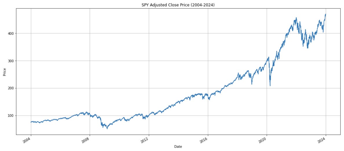
As of the date of writing the ETF Direxion Daily S&P500® Bull 3X Shares (SPXL) Performance has achieved a +10,084% return over the last 20 years, giving a CAGR of around 26.01%. Using the sample statistics of SPY returns, we plot the geometric growth rate against the leverage employed

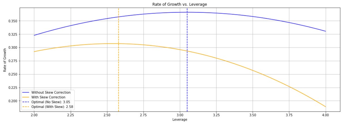
Note that optimal leverage with the skew correction (2.58) is indeed lower than optimal leverage without the skew correction (3.05) and that CAGR after accounting for skew (~31%) is lower than CAGR without accounting for skew (~36%). Realized CAGR (~26%) is lower than both, possibly because of kurtosis, management fees, and the cost of leverage. In any case, the results above accord with our intuition that accounting for negative skewness should decrease the optimal leverage as well as the expected growth rate of wealth.

Disclaimer

The information provided on TheLogbook (the "Substack") is strictly for informational and educational purposes only and should not be considered as investment or financial advice. The author is not a licensed financial advisor or tax professional and is not offering any professional services through this Substack. Investing in financial markets involves substantial risk, including possible loss of principal. Past performance is not indicative of future results. The author makes no representations or warranties about the completeness, accuracy, reliability, suitability, or availability of the information provided.

This Substack may contain links to external websites not affiliated with the author, and the accuracy of information on these sites is not guaranteed. Nothing contained in this Substack constitutes a solicitation, recommendation, endorsement, or offer to buy or sell any securities or other financial instruments. Always seek the advice of a qualified financial advisor before making any investment decisions.