Correlation is not Intuitive | Freeport Markets

From The Logbook. The original article is reproduced in full, with minor grammar corrections; references to market conditions reflect the context in which it was written.

We start with a short preference test that most readers, even practitioners, will answer incorrectly. The test and the following analysis are taken from Bridge Alt+’s article on Portfolio Intuition. We do a quick recap on Markowitz optimization and explore the implications of well-diversified portfolios on asset prices.

A Simple Exercise

Assume that you are a hedge fund manager with a portfolio that exhibits an excess return of 5% and a risk of 15% for a Sharpe ratio (excess return over risk) of 1/3. This is not as good as you’d like it to be so you are looking to allocate capital such that the resulting weights will be split 90% to your current portfolio and 10% to another asset. You want to improve your Sharpe ratio and you know that negatively correlated assets can help with that goal. The two assets you are presented with are:

As the fund manager, which one of these assets should you choose? Take a second to think about this carefully. The intuitive answer is clearly A1, but you are being asked by the author to consider your choice, so maybe adjust your priors. If you are familiar with mean-variance optimization, feel free to skip the next section and go straight to the solution.

Recap on Two-Asset Portfolio Optimization

We construct a portfolio p with assets A and B weighted by their corresponding weights. The expected return of the portfolio is given by the term

{E} (R_{p})=w_{A}{E} (R_{A}) + w_{B}{E} (R_{B})

The variance of the portfolio’s returns for that period is given by

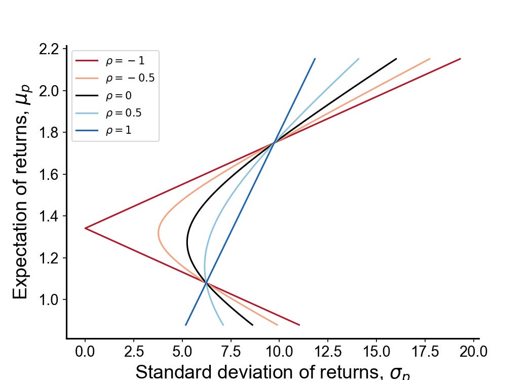
\sigma _{p}^{2}=w_{A}^{2}\sigma _{A}^{2}+w_{B}^{2}\sigma _{B}^{2}+2w_{A}w_{B}\sigma _{A}\sigma _{B}\rho _{AB}

Where Rho describes their correlation. Every possible combination of risky assets can be plotted in this risk-expected return space, and the collection of all such possible portfolios defines a region in this space. The left boundary of this region is hyperbolic, and the upper part of the hyperbolic boundary is the efficient frontier in the absence of a risk-free asset. The closer the correlation is towards -1, the more convex the efficient frontier. See below:

Solution to Initial Exercise

Since the returns of the A1 and A2 are identical, the returns of the resulting portfolio are indifferent to your choice.

We use the previously presented formula to calculate the risk for A1

We do the same for A2

From a mean-variance perspective, we should be indifferent to the choice between A1 and A2. Both assets produce a roughly 10% increase to the portfolio’s Sharpe.

Our intuitions strongly suggest that more risk, holding all else constant, is bad. While that is probably true in most scenarios, it doesn’t hold up when we are considering both the impacts of risk and correlation at the same time. If we look at the formula for the post-allocation risk S we see that there are two components of risk contribution from the added asset A, one which is quadratic and one which is linear. Under negative correlation, the linear term decreases with risk. See the combined effect:

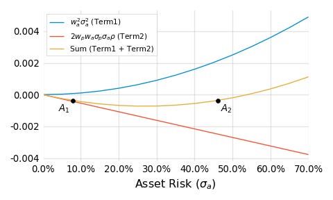
There are 2 observations to note. The first is that when adding a small amount of negatively correlated asset to a portfolio, the risks must be incredibly high before the performance of the resultant portfolio is degraded i.e. negative correlation makes an asset’s inclusion robust to risk. The second observation is that prior to the vertex of the quadratic, we have an area where added risk to the new asset has a positive payoff for the resultant portfolio i.e. reducing the Sharpe of the new asset increases the Sharpe of the resultant portfolio. These two observations are highly counter-intuitive; we now attempt to build a framework that resolves this issue.

Visualizing Indifference

But first, let’s consider a few more preference tests

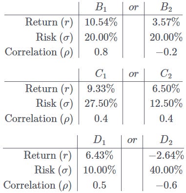
To make the exercise easier, we provide the risk-return plot of these assets

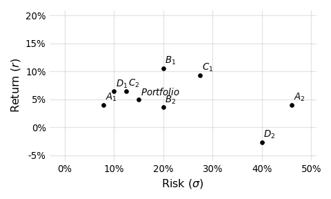
The punchline, of course, is that all the assets listed improve the Sharpe of the portfolio by 10%. Our intuition naturally likes assets on the upper left corner of lower risk and higher return. However, this vision is incomplete without considering correlation. We now present the same graph but with lines drawn to represent the effects of correlation structure. Each line drawn represents a class of assets that share the same correlation to the portfolio (0.8, 0.5, 0.4, -0.2, -0.6, from warm to cool colors) and deliver the same 10% improvement to the Sharpe ratio when allocated at 10%.

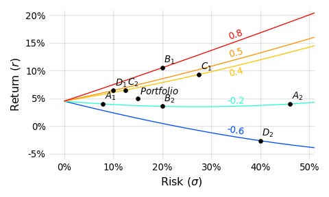
With the added lines we can see how as correlation drops, less return is required to deliver the same improvement in Sharpe. I hope that this exercise shows just how difficult it really is to internalize the effects of correlation, as well as how important it really is to portfolio performance.

Indifference Curves

We now aim to answer the question: “In terms of weighting, return, risk, and correlation, when am I indifferent to a new addition in my portfolio?” The answer to this question will help us answer the question of when it is desirable to add a new asset. The indifference curve can be written

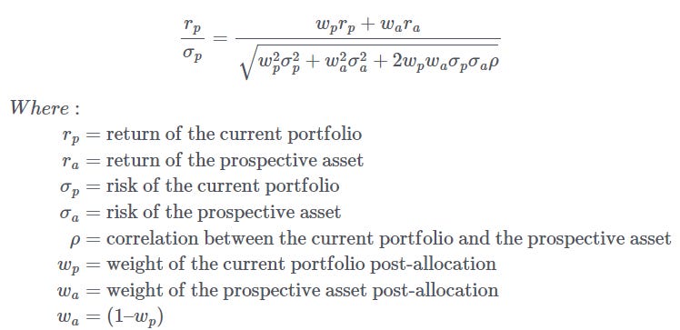
The LHS is the current Sharpe and the RHS is the Sharpe post addition of the new asset. We can now graph these indifference curves. The x-axis is the correlation between the new asset and the current portfolio, the y-axis is the Sharpe of the Asset divided by the Sharpe of the portfolio.

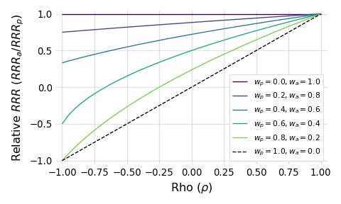
Each line represents an indifference curve between Sharpe ratio and correlation for a given weight. For example, the light green gives you the combination of correlations and Relative Sharpe (or Risk-Reward-Ratio in RRR) that you are indifferent to when you have allocated 20% of the original portfolio to the new asset.

As the weight allocated to the asset increases (lines going up from green to purple), the asset must have a higher Sharpe (relative to the portfolio) in order to do no harm. This should be intuitive since it says that as the impact of the asset on the portfolio increases, more is required of it since we lose more of the benefits of diversification.

The opposite also holds; the astute reader will note that as we shrink the weight allocated to the prospective asset, we reduce what’s required of it, and the limiting scenario (represented by the dashed line) gives the indifference equation

Very rarely do we encounter mathematical beauty in finance, but please do take a moment to appreciate the simplicity of this equation (before returning to reality and realizing that we do not live in a world of normally distributed returns). Just three terms (return, risk, correlation) are required to answer the question: “Does including a small amount of this asset add value to my portfolio?” Since we’d like to do better than merely being indifferent, we can change this into an inequality

\text{Sharpe}_a > \rho \times \text{Sharpe}_p

Interpreting Correlation

Correlation can be understood as a sort of performance hurdle. Indeed, for assets with zero correlation, marginal additions to your portfolio are always positive. The same is true for assets with Sharpe ratios greater than your portfolio, adding them will always help regardless of correlation. Unfortunately, there is no simple way to rank different assets except to brute force the Sharpe of different combinations.

An additional implication of high correlation, aside from a higher performance hurdle, is that it makes the weighting of assets more sensitive to the point estimates of mean, variance, and correlation itself. To elaborate, we have previously shown that given a risk-free asset and a risky asset, the optimal allocation (that which achieves the maximal geometric growth rate) towards the risky asset is equal to expected returns over variance. In the more general case of two risky assets we can show (on page 9) the optimal allocation is given by

w_1 = \frac{\mu_1 - \mu_2 + (\sigma_2 - \rho \sigma_1)\sigma_2}{\sigma_1^2 + \sigma_2^2 - 2 \rho \sigma_1 \sigma_2}

We can see that larger values of rho make w1 more sensitive to small perturbations in both rho itself as well as the other variables especially when we consider that for most assets sigma is much greater than mu. For example, in the case where asset 1 has 7% returns and 20% risk and asset 2 has 10% returns and 30% risk, the optimal allocation towards asset 1 has a highly non-linear relationship with correlation on the right

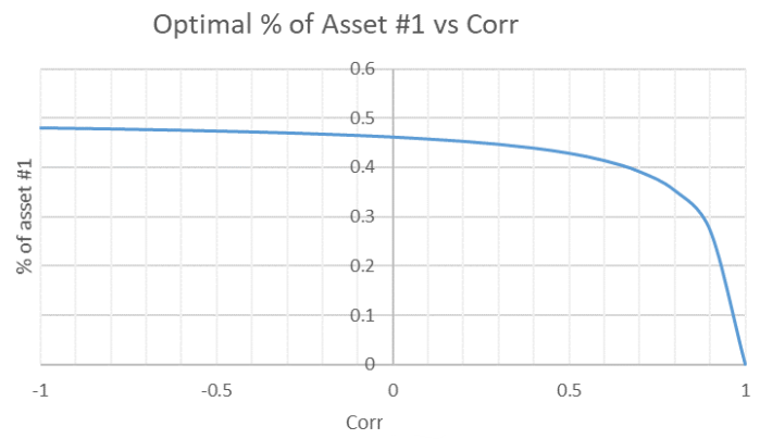
The graph here is taken from BreakingTheMarket’s article on the subject. An interesting result that he shows is that if two assets have the same geometric return, they should always be mixed in equal proportions regardless of arithmetic returns, risk, or correlation. For the purpose of this article, the point that we wish to make is that optimization in the context of high correlations is often difficult as it requires us to be more confident in our estimates of the moments of our assets. This is one of the reasons why running a mean-variance optimization algorithm on historical data will likely produce an overfitted portfolio that performs poorly in the real world; estimates of mean and variance from historical data are noisy and adversely impacts allocation decisions.

Implications for Diversification

Kris Abdelmessih has a blog post titled You Don’t See The Whole Picture that illustrates how correlation not only makes diversification good, but also necessary. He asks us to imagine a world with two stocks:

☀️Sunblock stock (SUN) makes 10% in sunny year. Loses 2% in rainy year.

☂️Umbrella stock (RAIN) loses 3% in sunny year. Makes 1% in rainy year.

Assume that the risk-free rate is 0 and that the year has a 50% chance to either be sunny or rainy. In isolation, it makes no sense to buy RAIN since it has an expected return of -1% versus SUN which has an expected return of 4%. Whatever the price of RAIN is, it would seem overvalued to the person who doesn’t know about SUN.

However, for those of us who can see the full picture, we note that the two stocks have -1 correlation and can see that even though SUN has a higher expected return and Sharpe than RAIN, a portfolio of 30% RAIN and 70% SUN even better (especially if we are allowed to leverage) since it is an arb. In short, assets that look overpriced in isolation can have rationally justifiable prices if they have some correlation with an unseen asset. In Kris’ words, “When you don’t understand the price you don’t understand the picture. The SUN/RAIN example shows how you would expect to lose money in RAIN in isolation because the market is priced assuming you buy SUN.”

Indeed, portfolio theory tells us that we do not get paid for diversifiable risks under reasonably efficient markets, since individual stocks themselves are unlikely to be on the efficient frontier. The price of assets is set by the buyer best equipped to take on its risk / the buyer where that asset is of the greatest value in their portfolio. The fact that a diversified portfolio will almost certainly have a higher Sharpe ratio than any individual asset implies that under fairly efficient markets, any standalone investment will be bid to the point where it’s “overpriced” when held in isolation. Put bluntly, if you are not diversifying to some extent, you are literally lighting money on fire in expectancy (although variance means that it is possible you over-perform).

The idea applies to trading as well. If someone is willing to pay me a high looking price, and I know that they aren’t retail, I need to think about the reason that they are so happy to pay me. For example, say that there’s been a surge in large cap single stock implied vol above what my models suggest, and I may now want to sell vol. But why is my counter party buying? They are, after all, sophisticated market makers. Perhaps if I checked index vol I will realize that they are selling correlation (long component vol short index vol) at over 100%. If I trade, I would be getting arbed. Maybe I am confident in my models and trade anyways, but now I at least know why the other side is willing to take the trade.