Asymmetric Vig Distribution | Freeport Markets

From The Logbook. The original article is reproduced in full, with minor grammar corrections; references to market conditions reflect the context in which it was written.

It is trivial to calculate implied probabilities when there is no bid-ask spread in the odds offered; however, a natural question arises when there is a spread as to where the true “mid-market” is. We show that under some reasonable assumptions, the Vigorish (also known as the juice, the cut, the take, the margin, the house edge, the spread, or the vig) charged by the bookmaker should be proportional to the fractional odds offered. When this is the case, the bookmaker is indifferent (on the margin) to which side of the book accumulates additional risk, and is also indifferent to which team the gambler’s private side information favors.

What Symmetric Vig Distributions Look Like

Naively one may think that in sportsbook pricing bookmakers would apply a uniform margin to their odds. That is, if the bookmaker adjusts one side of a market to 90% of its fair odds, the corresponding side (or multiple sides in multi-way markets) should be adjusted proportionally. For example, in point spreads and totals, many American bookmakers incorporate a margin of approximately 4.8%. Since these spreads are designed to reflect 50/50 odds, the odds are set by adding the margin to 100%, forming an overround. The fair probability is then multiplied by this overround to determine the breakeven win percentage for bettors:

50\% \times 104.8\% = 52.4\%

This calculation results in a line of -110 on both sides, since

100 \times \left(\frac{52.4\%}{52.4\% - 100\%}\right) \approx -110

More generally, in the case of two teams where one must win, and true probabilities are p and q respectively for team 1 and 2 (where p + q = 1), symmetric vig claims that given tradable probabilities of x and y (where x + y > 1) the relationship

p = \frac{x}{x+y}, \ \ \ \ \ q = \frac{y}{x+y}

holds generally. The vig here is symmetric since the percent profit the bookmaker makes per dollar that the gambler bets is equal on both teams. If the gambler buys team 1 then they pay x to get something that is worth x / (x+y), the percent profit is

\frac{x - \frac{x}{x+y}}{x} = \frac{x+y-1}{x+y} = \frac{y - \frac{y}{x+y}}{y}

which we see is equal to the percent profit in the case that the gambler buys team 2.

By structuring odds in this manner, the bookmaker ensures a consistent expected edge over bettors, irrespective of which side they wager on. Consequently, one would think the bookmaker remains indifferent to marginal imbalances in wagered amounts, as the expected value remains the same regardless of the distribution of bets. Indeed, this is in fact what many sport betting websites teach

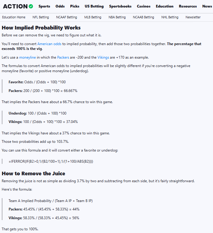
However, the conventional theory regarding sportsbook pricing has been challenged by empirical evidence. The examination of real sporting event outcomes, in comparison to the sharpest available closing lines, have demonstrated the presence of a favorite-longshot bias where a greater margin is placed on longshots by the bookmaker, while a smaller margin is applied to favorites. This observation raises two fundamental questions: how is the margin applied, and why would bookmakers accept a smaller edge on favorites while imposing a larger edge on longshots?

Why Vig Should be Asymmetric

Consistent expected edge over bettors irrespective of which side they wager on may seem like a desirable property for a book to have, but let us consider instead some other incompatible properties which may also be desirable.

We propose that a sportsbook acting as a market maker and potentially carrying financial risk from unbalanced betting action is not best served by maintaining an equal edge on both sides of a market; rather it is in the bookmaker’s best interest to remain indifferent to which side of a market carries excess risk under log-utility.

The same condition also ensures the maximum rate of growth for the wealth of the sports book for any risk that it does take on, an equal risk-reward ratio regardless of which side the bet is placed on, indifference of the sportsbook to which side the gambler’s private information favors (hence maximum edge in information space), and risk-free arbitrage by the sportsbook if the fraction of risk carried on each side is proportional to the fraction of growth-optimal risks (will explain this later). This condition is of course the Kelly-Optimal edge that the sportsbook should charge.

Deriving the Growth-Optimal Theoretical Odds

The Kelly Criterion seeks to maximize the long-term growth rate of wealth, this is equivalent to maximizing the expected logarithm of wealth (proof on Wikipedia) and equivalent to maximizing utility under a log-utility function. Suppose an individual starts with wealth W0 and bets a fraction f of their wealth on an outcome with probability p, where the net fractional odds are b. The final wealth after one bet is:

W = \begin{cases} W_0 (1 + f b), & \text{win with probability } p, \\ W_0 (1 - f), & \text{lose with probability } (1 - p). \end{cases}

Taking the logarithm of wealth:

\log W = \begin{cases} \log W_0 + \log (1 + f b), & \text{win}, \\ \log W_0 + \log (1 - f), & \text{lose}. \end{cases}

The expected logarithm of wealth growth is:

E(f) = p \log(1 + f b) + (1 - p) \log(1 - f).

For a sportsbook to be indifferent to the side that the marginal bet is applied to under log-utility means that the expected logarithmic growth for the favorite and the longshot must be the same i.e. where

E_1 = p \log(1 + f_1 b_1) + q \log(1 - f_1)

E_2 = q \log(1 + f_2 b_2) + p \log(1 - f_2)

we need to have

p \log(1 + f_1 b_1) + q \log(1 - f_1) = q \log(1 + f_2 b_2) + p \log(1 - f_2)

where

\begin{aligned} p, q &= \text{true probabilities of the favorite and longshot winning, respectively, where } p + q = 1. \\ f_1, f_2 &= \text{fraction of capital at risk for the favorite and longshot, respectively.} \\ b_1, b_2 &= \text{fractional odds for the favorite and longshot received by the sportsbook, respectively}. \end{aligned}

In particular, recall that the Kelly Criterion seeks to maximize the expected logarithm of wealth growth. For a single bet, the expected logarithmic growth function is:

E(f) = p \log(1 + f b) + (1 - p) \log(1 - f)

To find the optimal fraction f*, we differentiate with respect to f:

\frac{dE}{df} = \frac{p b}{1 + f b} - \frac{(1 - p)}{1 - f}

Setting this derivative to zero allows us to maximize expected growth, and after some algebraic manipulation we can show that

f^* = \frac{p b - (1 - p)}{b}

For a two-outcome market, we can then define the optimal fractions for betting on the favorite and the longshot:

f_1^* = p-\frac{q}{b_1}, \quad f_2^* = q-\frac{p}{b_2}

We can then solve for the true odds (isolating the term p/q) for both sides of the market (as a function of the implied probabilities of the posted odds) by assuming that the fractions of capital the bookmaker has at risk are (up to proportionality) the right optimal amount as prescribed by the above formulas so we can use the Kelly Criterion formula to substitute in odds and probabilities for the fractions f₁, f₂

p \left[ \log(1 + p b_1 - q) - \log(1 - q + p/b_2) \right] = q \left[ \log(1 + q b_2 - p) - \log(1 - p + q/b_1) \right]

Rearranging using log rules,

p \log\left(\frac{(1 + p b_1 - q)}{(1 - p + q/b_1)}\right) = q \log\left(\frac{(1 + q b_2 - p)}{(1 - q + p/b_2)}\right)

Substituting p + q = 1, and converting to implied probabilities using b = 1/p -1

p \log \left( \frac{1 - p_2}{p_1} \right) = q \log \left( \frac{1 - p_1}{p_2} \right)

Solving for the true odds ratio p / q

b_0 = p/q = \frac{\log (p_2 / q_1)}{\log (p_1 / q_2)}

\begin{aligned} p_1, p_2 &= \text{implied probabilities of the favorite and longshot, respectively.} \\ b_0 &= \text{true fractional odds of the longshot.} \\ 1/b_0 &= \text{true fractional odds of the favorite.} \end{aligned}

Properties of the Growth-Optimal Theoretical Odds

In a growth-optimal sportsbook, three key conditions are fundamentally linked: (1) the book is (roughly) balanced, meaning it is risk-free because it collects more in losing bets than it pays out in winning bets regardless of the outcome; (2) the money wagered on each side follows the Kelly-optimal ratio that maximizes long-term growth; and (3) the edge charged is proportional to the odds offered. Specifically, any two of these conditions necessarily imply the third.

If the sportsbook is balanced and the wager amounts align with Kelly-optimal proportions, then the edge must be structured proportionally to the odds. Conversely, if the book is balanced and the edge is proportional to the odds, then bettors would have placed their bets in Kelly-optimal proportions for the sportsbook. Lastly, if the wager amounts follow the Kelly-optimal fractions and the edge is proportional to the odds, then the sportsbook will end up balanced. We now outline the proof

(1) For the book to be balanced (i.e. risk-free arbitrage) we need

f_2 = f_1(1+b_1), \ \ \ \ \ f_1=f_2(1+b_2)

Since b1 = 1 / p1 - 1 and b2 = 1 / p2 - 1 the above is equivalent to

f_1 p_1 = f_2 p_2

(2) For the fractions wagered to be Kelly with respect to the true odds we need

f_1 = p-\frac{q}{b_1}, \quad f_2 = q-\frac{p}{b_2}

(3) For the vig collected to be proportional to odds received we need

\frac{p-p_1}{b_1} = \frac{q-p_2}{b_2}

We can show that (1) and (2) implies (3), and since the algebra involved is fully reversible it follows that any two of the conditions implies the third. Using (1) and (2) as well as the relationship between implied probability and fractional odds

p_1 = \frac{1}{1+b_1},\ \ \ \ \ p_2 = \frac{1}{1+b_2}

We can write that a balanced book which is also Kelly must satisfy

\left(p - \frac{q}{b_1} \right)p_1 = \left(q - \frac{p}{b_2} \right)p_2

Using p + q = 1 this can be re-written

\frac{(p(b_1+1)-1)p_1}{b_1} = \frac{(q(b_2+1)-1)p_2}{b_2}

Using the relationship between implied probability and fractional odds

\frac{(p(1/p_1)-1)p_1}{b_1} = \frac{(q(1/p_2)-1)p_2}{b_2}

Which simplifies to

\frac{p-p_1}{b_1} = \frac{q-p_2}{b_2}

as we set out to show. Again, since the algebra involved is fully reversible it follows that any two of the conditions implies the third.

Kelly-Optimal Odds Maximize Edge in Information Space

We assume now that the gambler has a small amount of private information which the sports book doesn’t have and show that the shift in fair probabilities is proportional to the fractional odds offered; a direct consequence is that only when edge is charged proportional to fractional odds is the sports book indifferent to the direction of the gambler’s private information, and hence maximizing edge in information space.

We consider Bayes' theorem, which show ups how to update the fair probability of an outcome O given new information I

P(O | I) = \frac{P(I | O) P(O)}{P(I)}

P(I) = P(I | O) P(O) + P(I | \neg O) P(\neg O).

The prior fair fractional odds of an outcome is given by

\text{Odds}(O) = \frac{P(O)}{P(\neg O)}

Doing some algebra, we see that Bayes' theorem gives us an elegant way of updating the odds using the likelihood ratio (right-most term below)

\text{Posterior Odds} = \text{Prior Odds} \times \frac{P(I | O)}{P(I | \neg O)}

This shows that the change in fair odds from n bits of information induces a change in that is proportional to the fair odds itself; i.e. a small shift in the probability of an outcome has a much larger impact on the fair odds for longshots compared to favorites. This is due to the convexity of the odds function, which “magnifies” changes in low-probability events.

This convexity matters because bettors with even modest informational edges on longshots see their expected value (EV) per unit risk increase dramatically, making longshots more exploitable when priced inefficiently. Conversely, for favorites, even with better information, the marginal gain in expected value is smaller, as the fair odds remain relatively stable to new information. This effect is key to understanding why sportsbooks often add greater margins to longshot compared to favorites bets to mitigate their exposure to informed bettors.

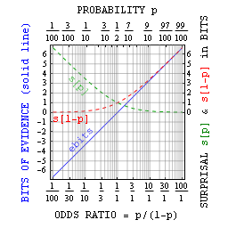
In the language of information theory, the convexity of odds transformations with respect to probability can be understood through the concept of self-information (surprisal), which quantifies how unexpected an event is. The surprisal of an outcome with probability p is given by I(p)=−log⁡2(p), meaning that as probability decreases, the amount of "information" contained in that event increases logarithmically. This function is convex, meaning that small changes in probability translate to disproportionately large changes in surprisal. The two primary strengths of surprisals are that they (i) reduce minuscule probabilities to numbers of manageable size, and (ii) add whenever probabilities multiply. Wikipedia explains this well

For example, one might say that "the number of states equals two to the number of bits" i.e. #states = 2^#bits. Here the quantity that's measured in bits is the logarithmic information measure mentioned above. Hence there are N bits of surprisal in landing all heads on one's first toss of N coins.

The additive nature of surprisals, and one's ability to get a feel for their meaning with a handful of coins, can help one put improbable events (like winning the lottery, or having an accident) into context. For example if one out of 17 million tickets is a winner, then the surprisal of winning from a single random selection is about 24 bits. Tossing 24 coins a few times might give you a feel for the surprisal of getting all heads on the first try.

More generally, one can relate probability p to bits of surprisal sbits as probability = 1/2^sbits, and with true-false assertions one can also define bits of evidence ebits as the surprisal against minus the surprisal for. This evidence in bits relates simply to the odds ratio = p/(1-p) = 2^ebits and shows why information affects fair odds so much more for smaller probabilities.

The average of surprisal over a distribution on is called its information entropy and the average difference of surprisals between distributions is called their Kullback–Leibler divergence. These ideas allow us to describe the general framework of the value of side information in betting (these are standard results in information theory which we will not prove here). Again, Wikipedia explains this well

A bit is the amount of entropy in a bettable event with two possible outcomes and even odds. Obviously we could double our money if we knew beforehand what the outcome of that event would be. However, no matter how complicated the betting scenario is, we can use an optimum betting strategy, called the Kelly criterion, to make our money grow exponentially with whatever side information we are able to obtain. The value of this "illicit" side information is measured as mutual information relative to the outcome of the bettable event

{\begin{aligned}I(X;Y)&=\mathbb {E} _{Y}\{D_{\mathrm {KL} }{\big (}P(X|Y)\|P(X|I){\big )}\}\\&=\mathbb {E} _{Y}\{D_{\mathrm {KL} }{\big (}P(X|{\textrm {side}}\ {\textrm {information}}\ Y)\|P(X|{\textrm {stated}}\ {\textrm {odds}}\ I){\big )}\},\end{aligned}}

where Y is the side information, X is the outcome of the betable event, and I is the state of the bookmaker's knowledge. This is the average Kullback–Leibler divergence, or information gain, of the a posteriori probability distribution of X given the value of Y relative to the a priori distribution, or stated odds, on X. Notice that the expectation is taken over Y rather than X: we need to evaluate how accurate, in the long term, our side information Y is before we start betting real money on X. This is a straightforward application of Bayesian inference. Note that the side information Y might affect not just our knowledge of the event X but also the event itself. For example, Y might be a horse that had too many oats or not enough water. The same mathematics applies in this case, because from the bookmaker's point of view, the occasional race fixing is already taken into account when he makes his odds.

The nature of side information is extremely finicky. We have already seen that it can affect the actual event as well as our knowledge of the outcome. Suppose we have an informer, who tells us that a certain horse is going to win. We certainly do not want to bet all our money on that horse just upon a rumor: that informer may be betting on another horse, and may be spreading rumors just so he can get better odds himself. Instead, as we have indicated, we need to evaluate our side information in the long term to see how it correlates with the outcomes of the races. This way we can determine exactly how reliable our informer is, and place our bets precisely to maximize the expected logarithm of our capital according to the Kelly criterion. Even if our informer is lying to us, we can still profit from his lies if we can find some reverse correlation between his tips and the actual race results.

Implications for Parlays

The convexity of odds in relation to probability shifts has implications for how sportsbooks collect edge on parlays. Since a parlay is simply the product of multiple individual bet odds, small shifts in implied probability (or also, implied correlation) at the single-bet level can compound dramatically when multiple legs are combined. Given that sportsbooks already bake in a margin on individual bets, this margin stacks exponentially across legs, leading to a disproportionate edge needed to justify the sportsbook’s risk on parlays compared to single bets.

Empirically, sportsbooks seem to recognizing this and do indeed back in higher margins. This explains why the most profitable sportsbook customers from a bookmaking perspective are often those who frequently bet longshot-heavy parlays; indeed, the Wall Street Journal reports that while 27% of cash wagered in Illinois, New Jersey, and Colorado in 2024 through October came in the form of parlays, these wagers accounted for 56% of revenue after payouts, showing that parlays (and small probability bets in general) are disproportionately profitable for bookmakers (and ought to be, in order to compensate the risk they are taking on both financially and in information space).

Recap

The analysis of sportsbook pricing under bid-ask spreads highlights that bookmakers should structure their vigorish (or "vig") proportional to the fractional odds offered. This ensures that the bookmaker remains indifferent to which side of the book accumulates risk and to the direction of any private information held by bettors.

The convexity of the odds function plays a central role in this analysis, as small shifts in probability have exponentially larger effects on longshot odds than on favorites. This convexity implies that bettors with modest informational edges on longshots can leverage their knowledge more effectively, making them more profitable at the expense of the bookmaker (if margins were symmetric). To counteract this, sportsbooks apply greater vig to longshots while reducing it for favorites.

The information-theoretic perspective further reinforces this structure, showing that the self-information (surprisal) of a rare event grows asymptotically as probability decreases. This explains why longshots are highly sensitive to new information and why even minor updates to their fair probability dramatically impact their implied odds. Using Bayesian updating, we see that information shifts in betting markets scale proportionally to the fractional odds offered, reinforcing the need for sportsbooks to scale vig proportionally as well.

This pricing model also extends naturally to parlays, where the bookmaker’s margin compounds across multiple legs due to the multiplicative nature of odds. Because each individual bet already incorporates vig, combining them exponentially increases the sportsbook's edge, leading to parlays being disproportionately profitable for bookmakers. Empirical data supports this, as sportsbooks generate far higher revenue shares from parlays than from straight bets, justifying their widespread promotion.

Ultimately, the growth-optimal sportsbook simultaneously achieves three key conditions: (1) a balanced book with risk-free arbitrage, (2) bet sizing that aligns with Kelly-optimal fractions, and (3) a vig structure proportional to fractional odds. Any two of these conditions necessarily imply the third, forming a mathematically consistent framework for sportsbook pricing. This ensures that sportsbooks maximize their long-term expected growth, remain indifferent to which side of a market attracts wagers, and extract maximum edge in information space from bettors operating with private signals.