Events & Forward Volatility | Freeport Markets

From The Logbook. The original article is reproduced in full, with minor grammar corrections; references to market conditions reflect the context in which it was written.

Earnings compress a large amount of uncertainty into a small amount of time. An option’s headline implied volatility blends events with ordinary diffusive volatility. Using the full surface, we can extract both the size of the announcement and the shape of its possible outcomes. This post explains what the term structure and curve reveal, as well as how major equity events ripples into other stocks.

Earnings Term Structure

An option containing an earnings event prices both variance accumulated over time as well as the separate earnings contribution. In notation we can write

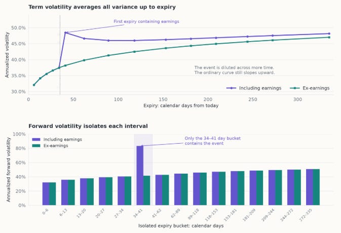
\sigma_{\text{total}}^2 = \sum_i \sigma_{\text{ordinary},i}^2 + \sigma_{\text{earnings}}^2

The first expiry containing earnings jumps above the ordinary curve. Subtracting adjacent variance budgets isolates the event in the 34–41 day bucket. The blue curve initially falls after that first event-containing expiry, then turns upward again, showing that the event is being diluted while the underlying ordinary-volatility curve slopes upward. It is straight forward to calculate forward volatility

\sigma_{\text{forward}} = \sqrt{ \frac{ \sigma_{\text{total},2}^2 - \sigma_{\text{total},1}^2 }{ T_2-T_1 } }

Interpolating ordinary variance between two surrounding expiries, then subtract it from the total variance, allows us to get a decent approximation at the earnings size. Where a and b are periods before and after the earnings expiry, we can approximate

\sigma_{\text{diffusive}} \approx \sqrt{ \frac{ \sigma_{\text{ordinary},a}^{2} + \sigma_{\text{ordinary},b}^{2} }{2} }

\sigma_{\text{earnings}} = \sqrt{ \left( \sigma_{\text{total}}^{2} - \sigma_{\text{diffusive}}^{2} \right)T }

Earnings Volatility Curve

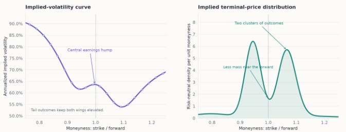
For European calls the Breeden–Litzenberger identity gives

q_T(K)=\frac{1}{D}\frac{\partial^2C(K,T)}{\partial K^2}

This shows that call-price curvature is proportional to the risk-neutral terminal-price density up to the reciprocal of the discount factor D. Typically, the recovered density has two dominant peaks which shows up as two dips in the vol curve

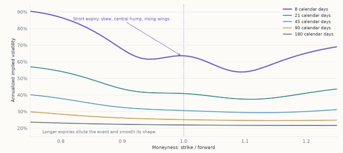
Longer expires makes the shape of earnings harder to identify as additional ordinary diffusion smooths its signature and dilutes its annualized contribution.

Earnings Print vs Guidance

The earnings print and the forward guidance from management deserve separate attention. EPS describes part of what happened while guidance, commentary and Q&A can change the expected path of cash flows for years. In general, earnings calls can happy 60-90 minutes after the initial print.

This is especially consequential on a Friday expiry; while options stop trading around 4PM ET most brokerages require exercise instructions by 5:30 PM ET. An intra-day release may also make the 0DTE options hard to price as the headline numbers may only contain a small percent of the uncertainty that the market expects to be resolved.

Suppose distant cash flows account for 35% of Company A’s present value and 80% of Company B’s. A 5% increase in those cash flows changes their values by 1.75% and 4%, respectively, holding discount rates and all else fixed.

Generally, guidance matter more for companies priced on distant growth. Higher P/E can be a clue but is an imperfect proxy as temporarily depressed earnings (often paired with low forward multiples) can also produce high present multiples.

Forecasting Earnings Size

Forecasting often begins with historical data then asks what has changed; in addition, pooling information from economically similar firms can make the estimates more stable. The option-implied event estimate is typically well-calibrated and efficient to within 15% of the most sophisticated estimates.

An under-appreciated fact (that sometimes creates dislocation) is that the condition of the market receiving the news matters. A company’s recent ordinary volatility may help predict its earnings reaction because it contains information about the order book’s capacity to absorb trading pressure.

Indeed, volatility itself can partly be explained through liquidity and order flow; as such, the same earnings surprise can elicit different responses depending on if it is naturally occurring in a period of shallow versus deep liquidity (of course, it is impossible to prove the counterfactual here). In other words, diffusive volatility and earnings moves are correlated.

Earnings Ripples

Earnings in one stock can often affect the price of different stocks. For example, the first memory producer to report can reveal something about industry pricing, inventory, customer demand or supply bottlenecks. A competitor therefore has part of the information in their own earnings revealed before their date.

These relationships change over time, but looking at stocks which are correlated diffusively is a good place to start (though the hyperscalers to semis ripple is a counterexample). The ripples are typically written as a beta to the main event:

r_B=\beta^{\mathrm{event}}_{B\leftarrow A}r_A+\varepsilon_B.

Analyst work typically supply the economic explanation. In general, stronger ripple effects are indeed observed for stronger economic links between firms. In rapidly changing / growing markets, ripples leave a lot of room for analysis to express skill.

While options-implied events estimates for earnings themselves are typically efficient to within 15% of the most sophisticated estimates, ripple sizes can be wildly mispriced (typically underpriced).

In addition, sometimes large ripple realizations should be vol-off for affected stocks depending on the reduction in expected surprisal from their subsequent earnings, but this effect is also often mispriced depending on analyst coverage.

Summary

We showed how to separate earnings risk from ordinary volatility using the term structure, and how the smile can reveal distinct outcome clusters. We discussed forecasting earnings moves through history, comparable companies, guidance and liquidity conditions. Finally, we noted how earnings ripple into related stocks, with changing economic links affecting both the immediate reaction and the uncertainty remaining around their own announcements.

Disclaimer: The information provided on TheLogbook (the “Substack”) is strictly for informational and educational purposes only and should not be considered as investment or financial advice. The author is not a licensed financial advisor or tax professional and is not offering any professional services through this Substack. Investing in financial markets involves substantial risk, including possible loss of principal. Past performance is not indicative of future results. The author makes no representations or warranties about the completeness, accuracy, reliability, suitability, or availability of the information provided.

This Substack may contain links to external websites not affiliated with the author, and the accuracy of information on these sites is not guaranteed. Nothing contained in this Substack constitutes a solicitation, recommendation, endorsement, or offer to buy or sell any securities or other financial instruments. Always seek the advice of a qualified financial advisor before making any investment decisions.