How to Extract Max Value from Your Edge?

From The Logbook. The original article is reproduced in full, with minor grammar corrections; references to market conditions reflect the context in which it was written.

How can you extract maximum value from a view that differs from the market, denominated in compound growth rate? In this post, we show that in any complete market, the maximum compound rate available equals the Kullback–Leibler divergence between their subjective measure P and the market’s risk-neutral measure Q, divided by time horizon. The payoff structure that achieves it is, up to scaling, is exactly the Radon–Nikodym derivative dP/dQ.

We consider a realistic example of 10% drift in equity index with a 2% risk-free rate. The numerical ceiling for max compound growth rate is around 14.5% above cash. A continuum of long calls or a continuously rebalanced ~312%-leveraged stock position achieves this exactly; a single five-year ATM LEAPS captures 93% of it. Information theory’s measure of statistical distinguishability turns out to be, in finance, the measure of value of an edge.

The material for this post was originally my final presentation for a graduate information theory course at university. Most of the mathematical results are drawn from existing literature, except the framing of single-LEAPS selection as a constrained KL projection with, which is my original mathematical contribution.

Introduction

This post walks through the question in a few steps.

(1) We set up the disagreement: the market prices under one measure Q, the trader believes another P, and we ask what the maximum extractable rate is given that gap.

(2) We solve the Kelly problem in a complete market and find that the growth-optimal payoff is, up to a constant, the likelihood ratio dP/dQ

(3) Plugging that payoff back into the objective shows that max growth rate is given by r + KL(P‖Q)/T i.e. value of an edge is its KL divergence from the market.

(4) We consider the special case of Black–Scholes, where dP/dQ becomes a clean power function of the terminal stock price, and show three different ways to actually trade it: a Carr–Madan continuum of long calls, a continuously rebalanced leveraged stock position, and a single call option.

(5) We frame single-option selection as a constrained KL projection, derive a tail-matching first-order condition for the optimal strike, and show that one ATM five-year call captures about 93% of the theoretical ceiling. The closing comparison plots terminal wealth distributions across all five strategies side by side.

Risk Neutral versus Real Distributions

As explained in one of my previous posts in greater detail, markets price contingent claims under a measure Q called the risk-neutral or martingale measure. Under Q, discounted asset prices are martingales, which is just the statement that option prices admit no arbitrage. The trader has a different belief, the physical or subjective measure P. If P = Q there is no edge. If P does not equal Q, there is an edge, and the question of this essay is: what is the maximum compound growth rate that edge can deliver, and what payoff structure realizes it?

Consider the following example with one risky asset under Black–Scholes:

\frac{dS_t}{S_t} = \mu \, dt + \sigma \, dW_t^P, \qquad S_0 = 100, \quad \mu = 0.10, \quad \sigma = 0.16

With risk-free rate r = 2% and trading horizon T = 5 years. The trader believes the drift is μ = 10%; the market prices options as if the drift were 2%. Volatility is agreed. The disagreement looks like this in the distribution of the asset S at time T:

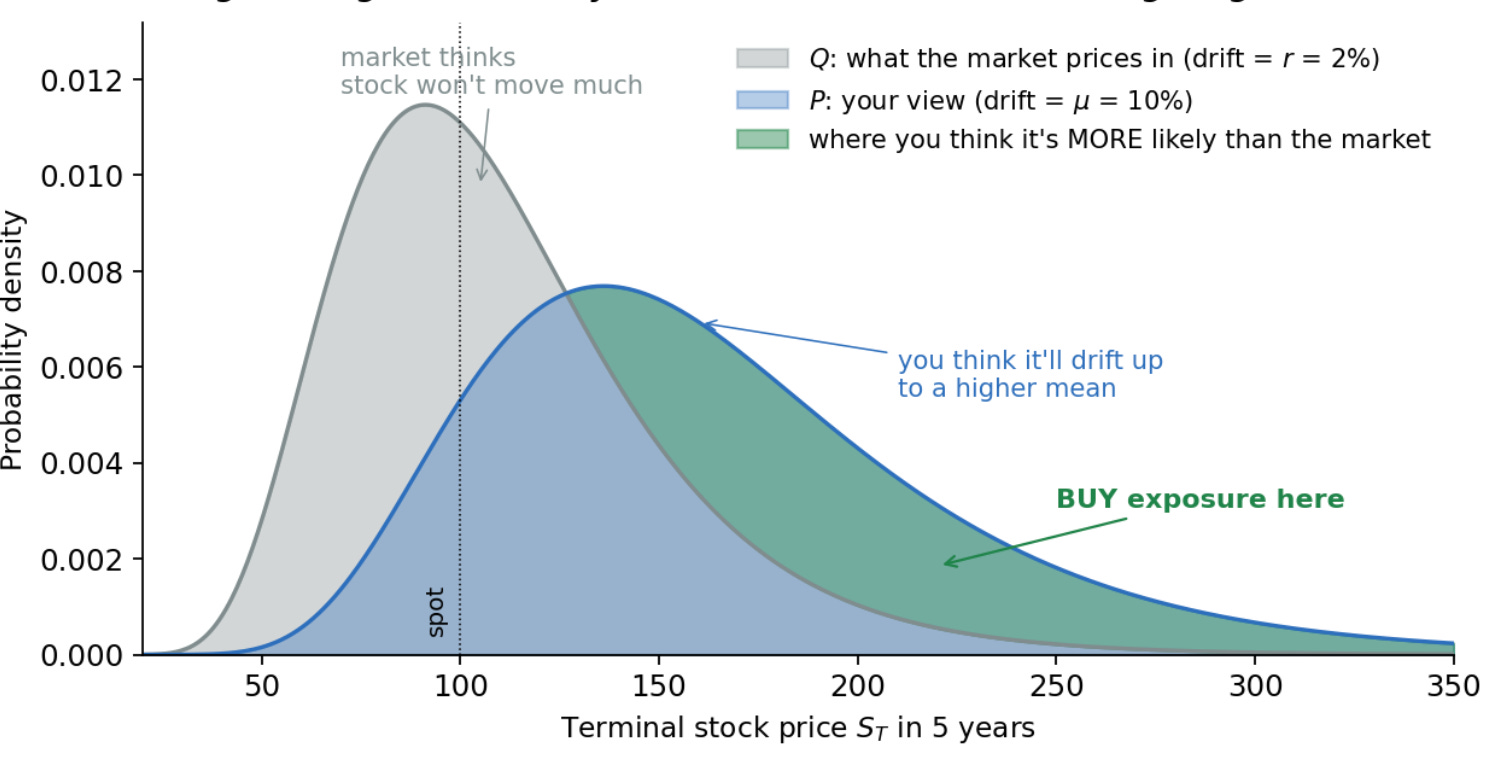
Both densities are lognormal with the same log-variance. Only the means differ:

E_Q[\log S_T] = \log S_0 + (r - \tfrac{1}{2}\sigma^2)T

E_P[\log S_T] = \log S_0 + (\mu - \tfrac{1}{2}\sigma^2)T

The trader’s distribution is shifted upward by (μ - r)T = 0.40 in log-units, putting more mass on outcomes above 126. Equivalently, the same Brownian motion produces different price paths under the two measures because the drift is different. Girsanov’s theorem makes this precise:

W_t^Q := W_t^P + \theta t

is a Brownian motion under Q, where

\theta := (\mu - r)/\sigma

is the market price of risk. For our parameters theta = 1/2.

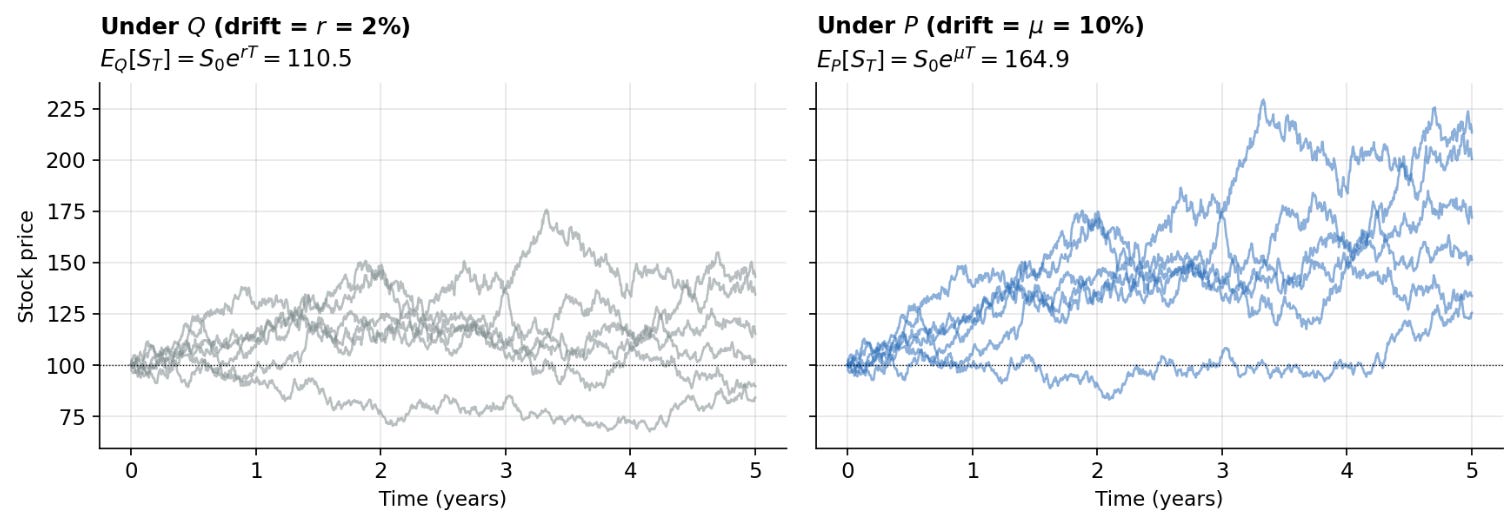
The two panels show six paths of the same underlying noise simulated under each drift. The shape of the noise is identical between the two, only the drift is different. Everything that follows can be read as: how much money is the trend gap worth, and what’s the cheapest way to extract it.

The Kelly Problem

Among all contingent claims W paying off at time T that cost W0 today, find the one that maximizes expected log-growth under the trader’s measure P:

\max_W \; E_P[\log W] \quad \text{subject to} \quad E_Q\!\left[W \cdot e^{-rT}\right] = W_0

The constraint is the no-arbitrage budget: every claim has a price, and that price is its Q-expected discounted value. The objective is the Kelly criterion (Kelly, 1956). Log utility is the right preference for compounding wealth because terminal wealth is multiplicative across reinvestment periods, so log is the unique utility for which one-period optimization gives the asymptotically growth-optimal strategy (Algoet and Cover, 1988). The market is assumed complete. We note that this is a constrained variational problem. Form the Lagrangian:

\mathcal{L}[W] = E_P[\log W] - \lambda \left( E_Q[W \cdot e^{-rT}] - W_0 \right)

Write the expectations as integrals against densities p and q. The Lagrangian becomes

\mathcal{L}[W] = \int p(s) \log W(s) \, ds - \lambda \int q(s) W(s) e^{-rT} \, ds + \lambda W_0

The first-order condition in W(s) (pointwise functional derivative) is

\frac{p(s)}{W(s)} - \lambda q(s) e^{-rT} = 0 \quad \Longrightarrow \quad W^*(s) = \frac{1}{\lambda e^{-rT}} \cdot \frac{p(s)}{q(s)}

Plug into the budget constraint to solve for λ:

W_0 = \int q(s) W^*(s) e^{-rT} \, ds = \frac{1}{\lambda} \int p(s) \, ds = \frac{1}{\lambda}

The optimal payoff is therefore

W^*(s) = W_0 \, e^{rT} \cdot \frac{p(s)}{q(s)} = W_0 \, e^{rT} \cdot \frac{dP}{dQ}(s)

This is the central object of the entire post. The growth-optimal contingent claim is, up to a constant, the Radon–Nikodym derivative dP/dQ. Where the trader’s density exceeds the market’s, the optimal payoff is large; where it is smaller, the optimal payoff is small. The optimal payoff is the likelihood ratio. (This is the classical duality solution to utility maximization; see Karatzas and Shreve, 1998, Ch. 3) Visualized for our example, dP/dQ as a function of S at time T looks like this:

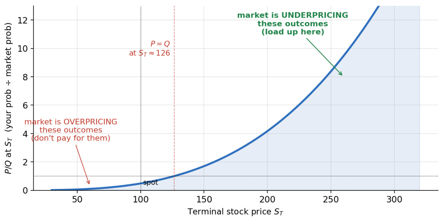
It is identically 1 at around 126 in our example (where P = Q), small below, and growing steeply above. The Kelly-optimal trade pays you a multiple of p/q at every state; implicitly it is telling us that we should load up where the market is underpricing and take nothing where it isn’t.

The Kullback-Leibler Divergence

Plug W* back into the objective:

E_P[\log W^*] = \log W_0 + rT + E_P\!\left[\log \frac{dP}{dQ}\right]

The Kullback–Leibler divergence of P from Q is defined as

D_{\text{KL}}(P \,\|\, Q) := E_P\!\left[\log \frac{dP}{dQ}\right] = \int p(s) \log \frac{p(s)}{q(s)} \, ds

So the maximum expected log-growth, divided by time, is

g^* = \frac{E_P[\log W^*] - \log W_0}{T} = r + \frac{D_{\text{KL}}(P \,\|\, Q)}{T}

This is a core result. The compound growth rate available to the optimal Kelly investor equals the risk-free rate plus the relative entropy rate between the trader’s view and the market’s. KL divergence, a purely information-theoretic object, is literally the value of the trader’s edge, denominated as a compounding rate.

Nothing about this part requires normality, continuous-time trading, or other Black–Scholes assumptions; it requires only a complete market and log utility. The original information-rate version of this result is in Kelly (1956); Cover and Thomas (2006, Ch. 16) develop the modern portfolio-theory restatement. The integrand tells you which stock outcomes contribute most to the divergence:

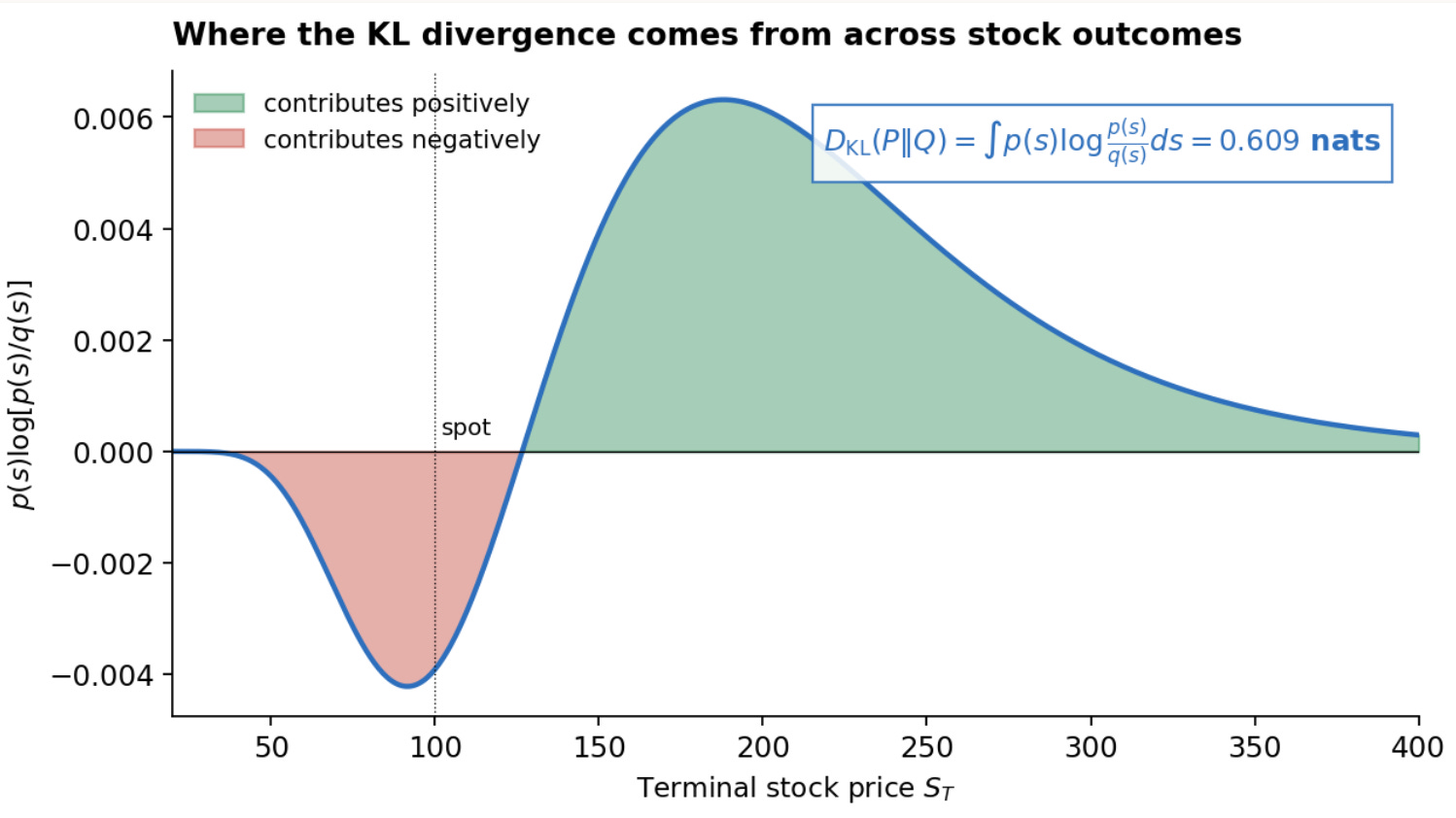
There is a negative region around spot, where p < q (the trader thinks these outcomes are less likely than the market), and a much larger positive region where p > q. The integral over the whole range is around 0.625 nats which gives around 14.5% max excess compounded annual returns attainable from the risk premium (note this is higher than the 8% risk premium from just buy and hold). We show this below.

Specializing to Black–Scholes

To compute the optimal payoff and growth rate explicitly in our example, we need dP/dQ as a function of S(T). Recall that the variance of these distributions are agreed-upon by both the trader and the market, and that only the means are different. Recall also that the density ratio of two same-variance normals is

\frac{f_P(x)}{f_Q(x)} = \exp\!\left( \frac{(x - m_Q)^2 - (x - m_P)^2}{2 \sigma^2 T} \right) = \exp\!\left( \frac{m_P - m_Q}{\sigma^2 T} \cdot \left(x - \tfrac{m_P + m_Q}{2}\right) \right)

\text{Substituting } x = \log s \text{ and } m_P - m_Q = (\mu - r)T

\frac{dP}{dQ}(s) = \exp\!\left(\frac{\mu - r}{\sigma^2} \cdot \log\frac{s}{C_0}\right) = c \cdot s^{\,\beta}, \qquad \beta := \frac{\mu - r}{\sigma^2}

for some normalizing constant c. The likelihood ratio in Black–Scholes is a power function in S(T). The exponent

\beta = \frac{\mu - r}{\sigma^2} = \frac{0.08}{0.0256} = 3.125

is the squared-Sharpe-per-variance which will reappear in three more places before we are done. The KL divergence has a closed form and can be computed directly using the lognormal moments:

D_{\text{KL}}(P \,\|\, Q) = \frac{(\mu - r)^2}{2 \sigma^2} \, T = \frac{1}{2}\theta^2 T

So the Black–Scholes Kelly–KL identity is

g^* - r = \frac{D_{\text{KL}}(P \,\|\, Q)}{T} = \frac{1}{2} \theta^2 = \frac{1}{2} \frac{(\mu - r)^2}{\sigma^2}

That is the hard ceiling. No strategy can beat it in expected growth rate. In our case

\tfrac{1}{2}(0.5)^2 = 0.125 \ \text{so} \ g^* = 14.5\%

The Optimal Payoff

We now substitute

dP/dQ \propto s^\beta

back into the optimal payoff formula so see that per dollar invested

W^*(s) = e^{rT} \cdot \frac{s^\beta}{E_Q[S_T^\beta]} = A \cdot s^\beta

where the normalization

A = e^{rT} / E_Q[S_T^\beta]

ensures the contract is priced at $1 today. The lognormal moment

E_Q[S_T^\beta] = S_0^\beta \exp(\beta r T + \tfrac{1}{2}\beta(\beta-1)\sigma^2 T)

is closed-form, giving

A = \frac{e^{rT}}{S_0^\beta \exp(\beta r T + \tfrac{1}{2}\beta(\beta-1)\sigma^2 T)} \approx 2.97 \times 10^{-7}

for our β = 3.125. So the Kelly-optimal payoff per dollar is approximately

W^*(S_T) = 2.97 \times 10^{-7} \cdot S_T^{3.125}

How does this compare to other strategies a trader might run? The chart below shows terminal wealth per dollar invested as a function of S at time T for five strategies:

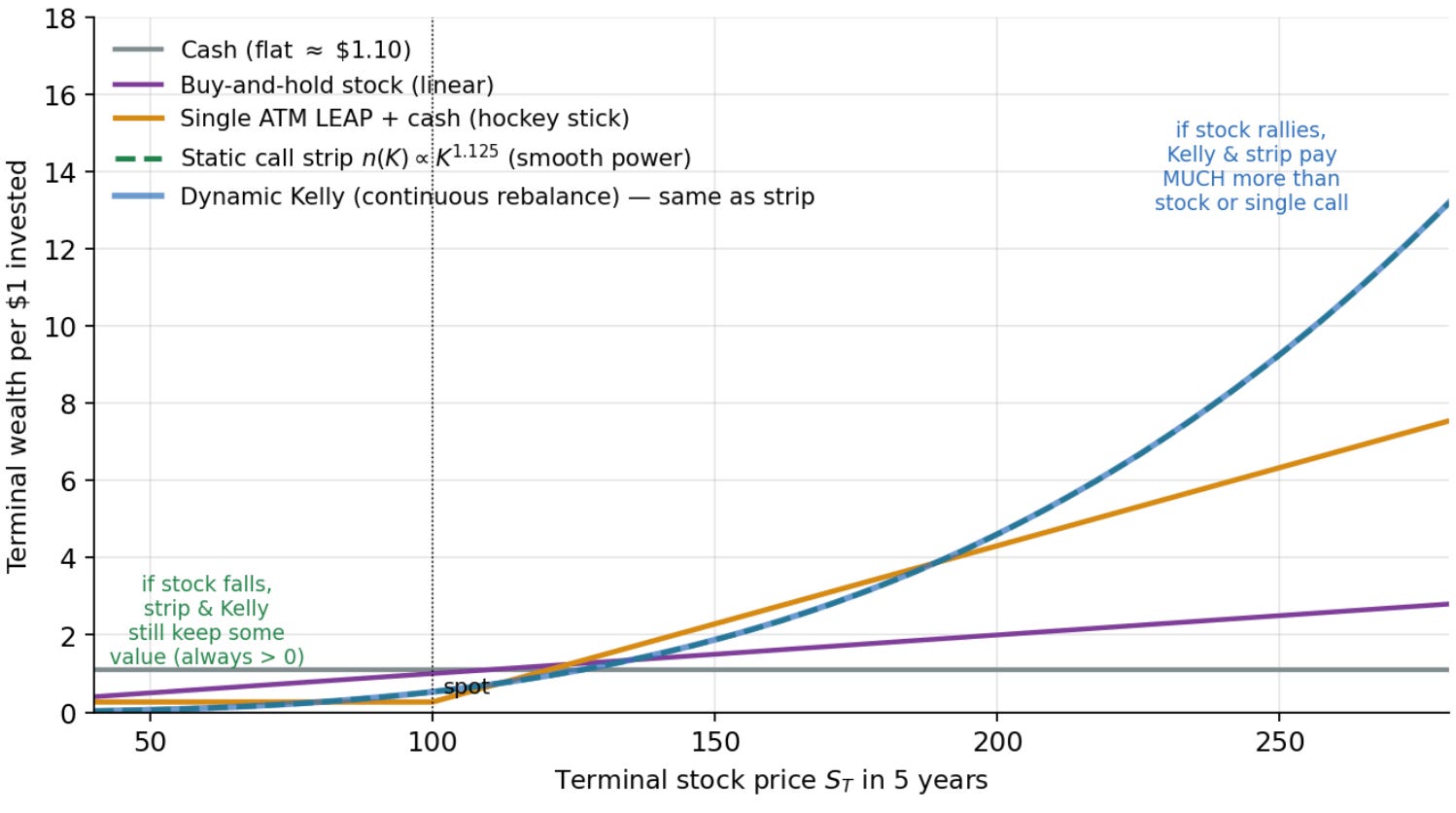
Cash is flat at around 1.10. Stock buy-and-hold is linear. A single ATM call plus cash is a hockey stick. The static call strip and dynamic Kelly are the same smooth power curve, plotted on top of each other. The strip and Kelly curves dominate single-stock and single-LEAPS aggressively in the upper tail, where the trader’s edge lives.

The LEAPS Call Approximation

Plot the integrand p(s) log W(s) for both the optimal payoff and ATM call:

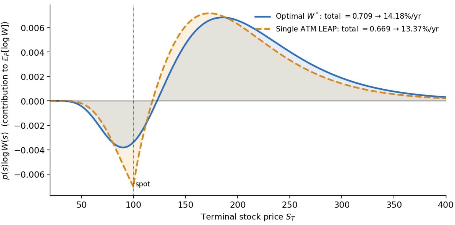
Both strategies generate negative contribution at low prices. Both also generate positive contribution in the upper tail. The differences is that the single call dips much further negative around 100 in the expired worthless region where the call paid nothing and you only have your cash residual. The optimal payoff is positive everywhere above roughly 130 and tracks the call closely from there up. There is however still a slight difference in the area between the curves. This is what the edge lost by suboptimal execution looks like geometrically.

Implementing W* with Vanilla Calls

The optimal payoff W* is an exotic and doesn’t trade. To realize it, the trader has to build it from instruments that do trade. The Carr–Madan static replication theorem says that for any twice-differentiable payoff H(S) with H(0) = H’(0) = 0, the identity

H(s) = \int_0^\infty H''(K) \, (s - K)^+ \, dK

decomposes H as a portfolio of long calls. The proof is integration by parts:

\int_0^s H''(K)(s - K) \, dK = H(s) - H(0) - s H'(0) = H(s)

when the boundary terms vanish. In our case

W^*(S_T) = A \cdot S_T^\beta, \ H^*(s) = A \cdot s^\beta

Differentiating twice shows that the Kelly-optimal portfolio holds calls at strike K with density

H^{*\prime\prime}(K) = A \beta (\beta - 1) K^{\beta - 2}

For our example

\beta - 2 = 1.125, \ n(K) \propto K^{1.125}

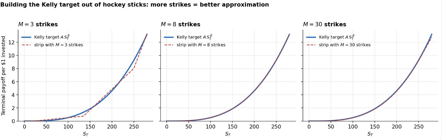
This shows that the further out of the money, the more contracts. (Each individual deep-OTM call is cheap; you can afford a lot of them per dollar.) The complete portfolio is a continuum of long calls; no stock, no puts, no cash. The replication identity is due to Carr and Madan (1998). We can observe convergence to the exact target as we increase the number of strikes:

The contract density keeps rising with the strike but individual call prices fall fast. So the capital density i.e. dollars deployed per unit strike is actually hump-shaped:

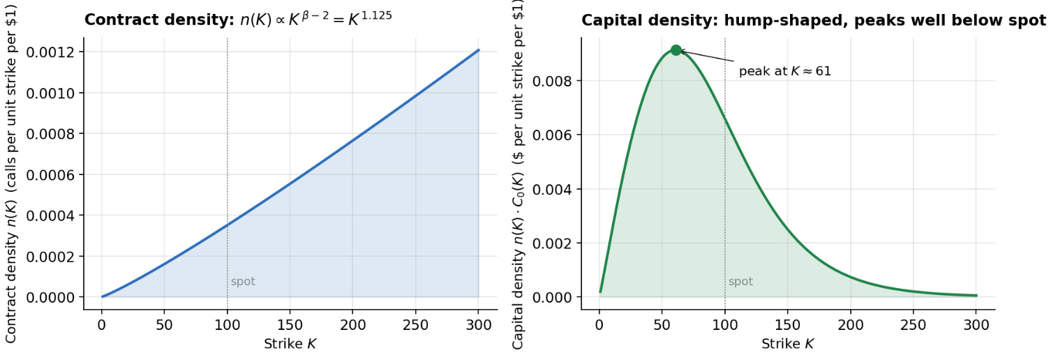
Most of the dollars go into a broad mid-strike region peaking around 60, well below spot, even though the contract count is heaviest in the wings.

Single LEAP as a Constrained Projection

In practice traders rarely buy a 30-strike strip. The realistic question is: given that you’re going to buy one call, which strike, and how much of your bankroll? This is a constrained version of the Kelly problem. Restrict the admissible payoffs to the two-parameter family generated by a call at strike K plus cash with fraction f in the call:

W_{f, K}(S_T) = (1 - f) e^{rT} + f \cdot \frac{(S_T - K)^+}{C_0(K)}

where

C_0(K) = E_Q[(S_T - K)^+ \cdot e^{-rT}]

is the Black–Scholes call price. The normalized payoff

Z_K := (S_T - K)^+ / E_Q[(S_T - K)^+]

satisfies

E_Q[Z_K] = 1

implying that strategy W satisfies

E_Q[W_{f,K} \cdot e^{-rT}] = 1

Note that

C_0(K) = e^{-rT} E_Q[(S_T-K)^+]

implying

(S_T - K)^+/C_0(K) = e^{rT} Z_K

which gives

W_{f,K} = e^{rT} \cdot [(1-f) + f Z_K] = e^{rT} \cdot [1 + f(Z_K - 1)]

Define the call-induced measure tilt Q by

\frac{dQ_{f, K}}{dQ} := W_{f, K} \cdot e^{-rT} = 1 + f(Z_K - 1)

which we can show to be a valid probability measure (proof left as an exercise to the Substack reader). The expected log-growth under P is

G(f, K) = E_P[\log W_{f, K}] = \log(e^{rT}) + E_P\!\left[\log \frac{dQ_{f, K}}{dQ}\right]

Apply

\log(dP/dQ_{f, K}) = \log(dP/dQ) - \log(dQ_{f, K}/dQ)

to calculate the expectation as

D_{\text{KL}}(P \,\|\, Q_{f, K}) = D_{\text{KL}}(P \,\|\, Q) - E_P\!\left[\log \frac{dQ_{f, K}}{dQ}\right]

Combining the above gives

G(f, K) - rT = D_{\text{KL}}(P \,\|\, Q) - D_{\text{KL}}(P \,\|\, Q_{f, K})

In words, the result shows that choosing the strike and position size of a single call is exactly the problem of finding the call-generated probability measure closest to the trader’s true measure in KL divergence. The 2D landscape of G over the full (K, f)-space looks like this:

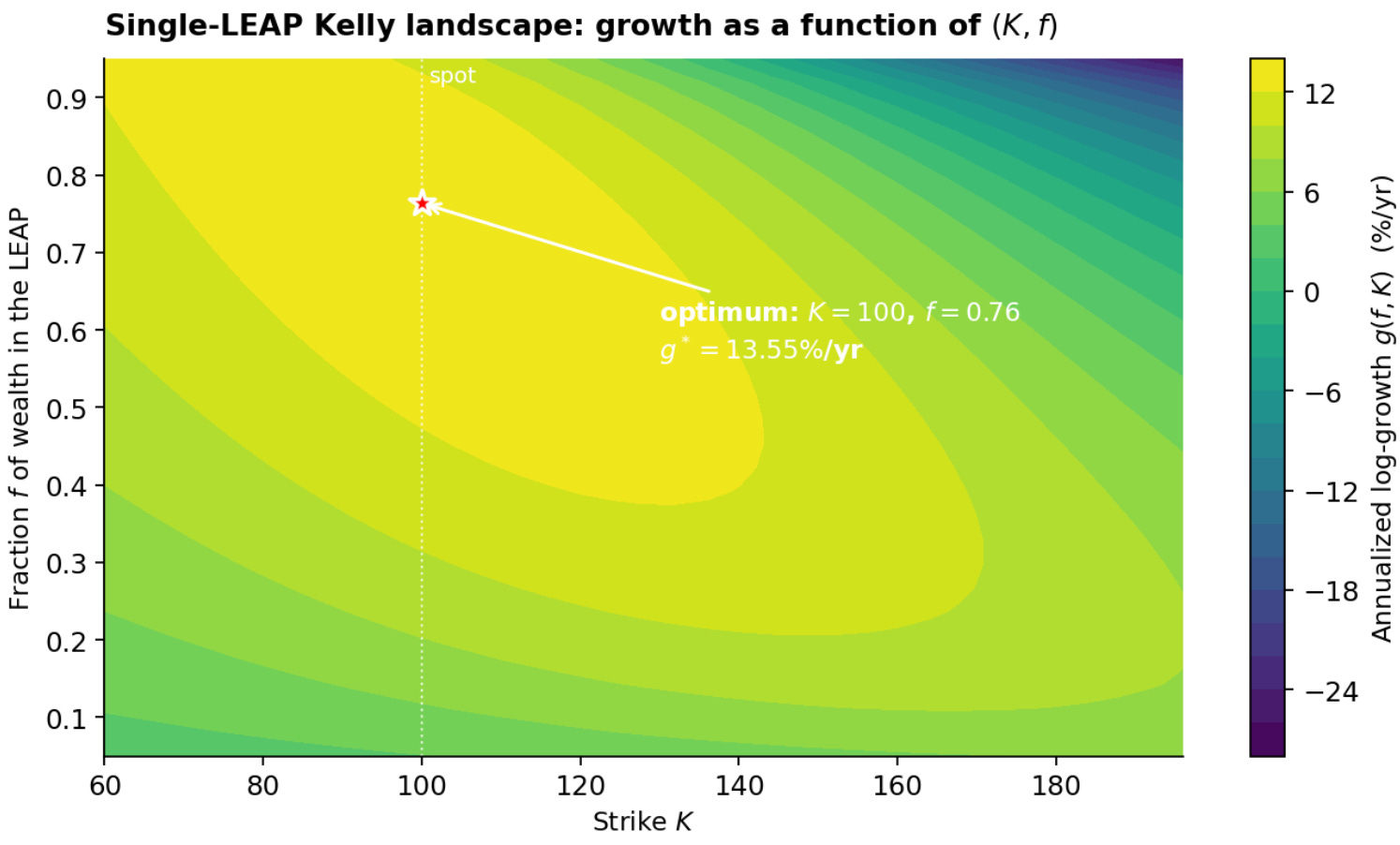
The maximum is in the upper-left region, with f approximately being 0.76 at strikes near spot, and decays smoothly in all directions. The optimum achieves roughly 13.55% excess returns a year. Cutting along the optimal f*(K) ridge gives the one-dimensional growth profile:

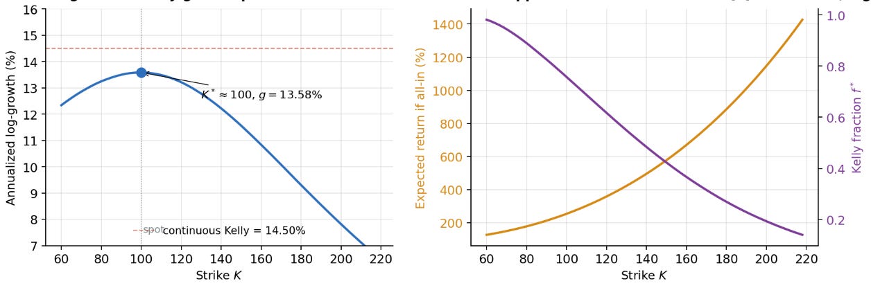
From the left, we see that the peak is around 100 numerically and the curve is broad such that anywhere from 90 to 110 delivers within 10 bps of optimal. The right panel shows two opposing recommendations under different objectives: linear expected return (orange) grows monotonically with K because deeper-OTM calls have higher payoff multiples, while the optimal Kelly fraction (purple) falls because log utility punishes the rising probability of finishing worthless.

The first-order condition for the optimal strike also has a clean form. Differentiating G in K (envelope theorem on the inner f-optimization) and using

\partial_K (S_T - K)^+ = -\mathbf{1}\{S_T > K\}

gives, after simplification

Q(S_T > K^*) = \widetilde{P}_{K^*}(S_T > K^*)

where the right hand side is the physical measure tilted by

1/(1 + f^*(K)(Z_K - 1))

Thus, the optimal strike is the one where the risk-neutral digital probability of finishing in the money matches a Kelly-tilted physical digital probability. There is no closed-form solution; it must be solved numerically, and the answer is parameter-dependent. ATM is NOT generically optimal, it just happens to be near-optimal under “reasonable” parameters.

Why a Single Call Works

The reason a static long call does so well, capturing 93% of the dynamic Kelly edge with one trade, is convexity. Under Black–Scholes, the dynamics of any option price can be derived by Itô’s Lemma. Starting from the BS PDE

\partial_t C + r S \partial_S C + \tfrac{1}{2} \sigma^2 S^2 \partial_S^2 C = r C

and applying Itô to C under P:

dC = \left[r C + (\mu - r) S \partial_S C \right] dt + \sigma S \partial_S C \, dW_t^P

Dividing by C and writing

\Omega := S \partial_S C / C

for the call’s elasticity (also called leverage or lambda) shows

\frac{dC}{C} = \left[r + \Omega (\mu - r)\right] dt + \Omega \sigma \, dW_t^P

Omega is equal to the Spot times Delta divided by the Call price and measures the option’s elasticity / leverage i.e. the percentage move in the option price per 1% move in the stock. If the stock rises 1%, an option with Omega = 5 rises 5%. ATM short-dated options typically have Omega in the 10–30 range; deep ITM options have Omega near 1; deep OTM options can have Omega in the hundreds.

Three observations. First, the option’s expected excess return is Omega times (mu − r) and its volatility is Omega times sigma, so the instantaneous Sharpe ratio is exactly (mu − r) / sigma which is the same as the stock. Second, Omega varies with the underlying: Omega = S · Delta / C and as the stock rises, Delta rises (due to positive Gamma everywhere). Third, in the continuous-rebalancing limit at Kelly fraction is (mu − r) / (Omega² · sigma²) for an option, the achievable growth rate r + (1/2) · (mu − r)² / sigma² is strike-independent.

For a static long call, the leverage profile Omega(S) does the work that dynamic rebalancing would have to do explicitly. As S rises the position naturally levers up; as S falls it de-levers. This is “synthetic momentum trading” baked into the contract. But the profile is fixed by the Black–Scholes formula and is concentrated near the strike. The Kelly-optimal target is a smooth power that grows without bound. A single call’s Delta(s) is a sigmoid that saturates at 1 once s is far ITM.

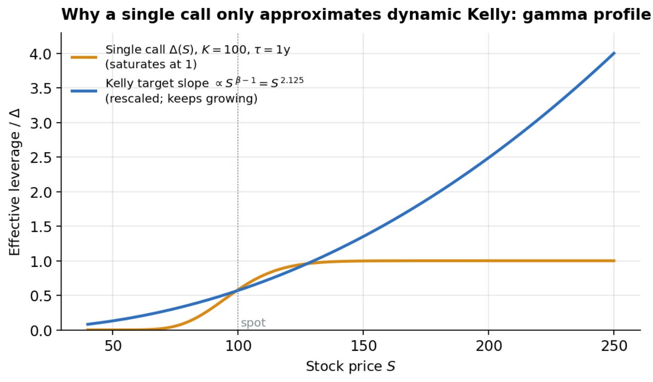
The orange call delta approaches 1 and saturates around 130, after which the call cannot lean any further into a continued rally. The blue Kelly target slope has no such ceiling. However, note that a single call gets ~93% of it because the orange and blue curves agree in the middle of the action around the 80 to 140 range where most of the distribution lives anyways, and only diverge in the deep tails.

The Dynamic Alternative

There is a third way to realize the optimal payoff, neither static-call-strip nor single-LEAP. Hold no options at all; instead, continuously rebalance a position in the underlying stock. I have written about this before. Let pi be the fraction of wealth in stock and 1 - pi in the risk-free asset, rebalanced continuously. Wealth dynamics are

\frac{dW_t}{W_t} = r \, dt + \pi \left[ \frac{dS_t}{S_t} - r \, dt \right] = \left[ r + \pi (\mu - r) \right] dt + \pi \sigma \, dW_t^P

Apply Itô to log W

d \log W_t = \left[ r + \pi (\mu - r) - \tfrac{1}{2} \pi^2 \sigma^2 \right] dt + \pi \sigma \, dW_t^P

Maximizing the drift over pi gives the Kelly fraction

\pi^* = \frac{\mu - r}{\sigma^2} = \beta = 3.125

The maximum drift is

r + \tfrac{1}{2} (\mu - r)^2 / \sigma^2

the same expression as the KL bound. That is the third place beta appears: as the optimal leverage. This is the log-utility special case of the classical Merton fraction (Merton, 1969); see also Long (1990) for the numéraire-portfolio interpretation. To see what terminal wealth this strategy produces, integrate d log W

\log \frac{W_T}{W_0} = \left[ r + \pi^* (\mu - r) - \tfrac{1}{2} (\pi^*)^2 \sigma^2 \right] T + \pi^* \sigma \, W_T^P

The Brownian term on the very right hand side is recoverable from the stock SDE

\log(S_T / S_0) = (\mu - \tfrac{1}{2} \sigma^2) T + \sigma W_T^P

\sigma W_T^P = \log(S_T / S_0) - (\mu - \tfrac{1}{2} \sigma^2) T

Substituting and simplifying

\log \frac{W_T}{W_0} = (1 - \pi^*) \left( r + \tfrac{1}{2} \pi^* \sigma^2 \right) T + \pi^* \log \frac{S_T}{S_0}

Equivalently

W_T = W_0 \cdot c_T \cdot \left( \frac{S_T}{S_0} \right)^{\pi^*}, \qquad c_T = \exp\!\left[ (1 - \pi^*) (r + \tfrac{1}{2} \pi^* \sigma^2) T \right]

The dynamic Kelly strategy produces a terminal wealth that is a deterministic function of the terminal stock price under Black-Scholes assumptions. Note that even if the stock ends where it started, continuous Kelly loses money because holding leverage constant forces buying after rallies and selling after drawdowns, skimming wealth on every round trip through volatility. The fact that final wealth depends only on the terminal state (and not the path) is purely an artifact of the assumption that rebalancing is continuous and costless; in practice, even daily rebalancing introduces meaningful path dependence.

Conclusions

Comparing terminal wealth distributions across paths, with each strategy’s bin masses normalized so they sum to 100%

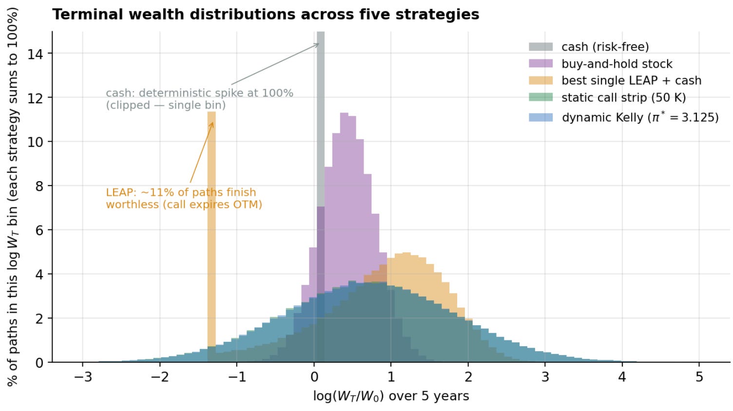
Cash is a delta function (the clipped 100% spike). Buy-and-hold stock gives a tighter lognormal that is moderately wider than cash but with much less upside than the option strategies. Single LEAP has a discrete probability mass near from expired worthless paths (~11% of the time) plus a smooth right-tail distribution that dominates buy-and-hold stock for most upside outcomes.

Strip and dynamic Kelly are visually identical broad smooth distributions, exactly as predicted by their being mathematically identical contracts. The Kelly/strip distributions are wider than the call in both directions, they pay much more on the upside but also leave you with less than the call when the stock falls hard, because the leverage embedded in the convex payoff cuts both ways.

Reading across the derivation, the key results are:

\text{Optimal payoff:} \quad W^*(s) = W_0 \, e^{rT} \cdot \frac{dP}{dQ}(s)

\text{Optimal growth:} \quad g^* - r = \frac{1}{T} D_{\text{KL}}(P \,\|\, Q)

\text{Black-Scholes special case:} \quad \frac{dP}{dQ}(s) \propto s^{\beta}, \quad \beta = \frac{\mu - r}{\sigma^2}, \quad g^* - r = \frac{1}{2} \frac{(\mu - r)^2}{\sigma^2}

\text{Static call replication:} \quad n(K) = A \beta (\beta - 1) K^{\beta - 2}, \quad A = \frac{e^{rT}}{E_Q[S_T^\beta]}

\text{Dynamic strategy:} \quad \pi^* = \beta, \quad W_T = W_0 \, c_T \, \left( S_T / S_0 \right)^{\beta}

\text{Single-LEAPS projection:} \quad G(f, K) - rT = D_{\text{KL}}(P \,\|\, Q) - D_{\text{KL}}(P \,\|\, Q_{f, K})

Note that the identity

g^* - r = D_{\text{KL}}(P \,\|\, Q) / T

is distribution-free. It does not require normality, continuous-time trading, or any specific market model. It says: in a complete market, the maximum compound growth rate equals the relative entropy rate between the trader’s measure and the market’s.

Whatever the source of the trader’s edge, fundamental research, alternative data, microstructure, behavioral views, its dollar value as a continuous compounding rate is the KL divergence. What you are paid for is distinguishability which is measurable from an information theory point of view.

The optimal payoff is always the likelihood ratio dP/dQ. Black–Scholes is the special case where the answer is a power function and a stack of calls reproduces it.

References

The Kelly criterion and the information-theoretic value of an edge

Kelly (1956), “A New Interpretation of Information Rate,” Bell System Technical Journal 35(4): 917–926.

The original paper. Introduces the log-optimal capital-growth rule and proves that for fair-odds gambling, the maximum exponential rate at which capital can compound equals Shannon’s information rate, the foundational form of the identity between an information-theoretic quantity (rate at which a signal carries information) and a financial quantity (rate at which wealth grows).

Cover & Thomas (2006), Elements of Information Theory, 2nd ed., Wiley, Ch. 16.

The standard modern textbook treatment. Generalizes Kelly’s result from horse-race gambling to log-optimal portfolios in arbitrary asset distributions, identifies the maximum compound growth rate with the relative entropy between the trader’s distribution and the market’s, and shows that the optimal portfolio weights are proportional to the trader’s probability over the market’s at each state.

Algoet & Cover (1988), “Asymptotic Optimality and Asymptotic Equipartition Properties of Log-Optimum Investment,” Annals of Probability 16(2): 876–898.

Proves that the log-optimal strategy is asymptotically optimal in a strong path-by-path sense, not just on average, no causal investment strategy can outperform it in the long run, regardless of the underlying return process. Justifies why log utility (rather than any other utility) is the privileged criterion when wealth compounds.

Bell & Cover (1980), “Competitive Optimality of Logarithmic Investment,” Mathematics of Operations Research 5(2): 161–166.

Establishes a separate optimality property of the log-optimal strategy: it cannot be beaten in head-to-head wealth comparisons more than half the time, against any opposing strategy. A third angle on why log utility is special.

Optimal payoff and the likelihood ratio (utility-maximization duality)

Karatzas & Shreve (1998), Methods of Mathematical Finance, Springer, Ch. 3.

The cleanest textbook derivation of the martingale/duality method: maximizing expected utility of terminal wealth subject to the no-arbitrage budget constraint reduces to a one-dimensional Lagrangian, with the optimal contingent claim equal to the inverse marginal utility evaluated at a multiple of the market’s likelihood ratio. For log utility this collapses to the optimal terminal wealth being proportional to the trader’s probability density divided by the market’s.

Kramkov & Schachermayer (1999), “The Asymptotic Elasticity of Utility Functions and Optimal Investment in Incomplete Markets,” Annals of Applied Probability 9(3): 904–950.

Generalizes the duality / likelihood-ratio characterization of optimal investment to general semimartingale markets, including incomplete ones, and establishes the conditions on utility functions (”asymptotic elasticity”) under which a clean duality solution exists.

Continuous-time portfolio choice (the Kelly fraction)

Merton (1969), “Lifetime Portfolio Selection under Uncertainty: The Continuous-Time Case,” Review of Economics and Statistics 51(3): 247–257.

Derives, for the first time in continuous time, the optimal constant fraction of wealth to hold in a risky asset. For a log-utility investor in a Black–Scholes economy the answer is the asset’s excess return divided by its variance.

Merton (1971), “Optimum Consumption and Portfolio Rules in a Continuous-Time Model,” Journal of Economic Theory 3(4): 373–413.

Extends to multiple risky assets, giving the optimal vector of asset weights as the inverse covariance matrix times the vector of excess returns over cash.

Change of measure (Girsanov) and the closed-form KL divergence in Black–Scholes

Karatzas & Shreve (1991), Brownian Motion and Stochastic Calculus, 2nd ed., Springer GTM 113, Section 3.5.

The rigorous probability-theory treatment of Girsanov’s theorem, the result that lets you change the drift of a Brownian motion by switching probability measures, with an explicit formula for the likelihood-ratio process between the two measures.

Static replication of nonlinear payoffs (Carr–Madan)

Carr & Madan (1998), “Towards a Theory of Volatility Trading,” in R. A. Jarrow, ed., Volatility: New Estimation Techniques for Pricing Derivatives, Risk Books, pp. 417–427.

Establishes the static replication identity that any twice-differentiable European payoff can be written as a weighted integral over strikes of vanilla call payoffs, with the weight at each strike equal to the second derivative of the target payoff.

The numéraire portfolio (the power-curve payoff)

Long (1990), “The Numéraire Portfolio,” Journal of Financial Economics 26(1): 29–69.

Introduces the numéraire portfolio: a self-financing trading strategy whose value, when used as the unit of account, makes the discounted prices of all other assets into martingales without any change of measure. In a Black–Scholes economy the numéraire portfolio’s value is proportional to the stock price raised to a power equal to the excess return divided by the variance.

Disclaimer

The information provided on TheLogbook (the “Substack”) is strictly for informational and educational purposes only and should not be considered as investment or financial advice. The author is not a licensed financial advisor or tax professional and is not offering any professional services through this Substack. Investing in financial markets involves substantial risk, including possible loss of principal. Past performance is not indicative of future results. The author makes no representations or warranties about the completeness, accuracy, reliability, suitability, or availability of the information provided.

This Substack may contain links to external websites not affiliated with the author, and the accuracy of information on these sites is not guaranteed. Nothing contained in this Substack constitutes a solicitation, recommendation, endorsement, or offer to buy or sell any securities or other financial instruments. Always seek the advice of a qualified financial advisor before making any investment decisions.