


Most of the theoretical results in this post are taken from a paper titled “An Asset Allocation Primer” published by PIMCO Quantitative Research in October 2017.
Leveraged ETFs
Leveraged ETFs often get a bad rap — labeled as tools only for gamblers or day traders (see Bloomberg posts below, for example).


But when you look deeper, their use (especially on well-diversified indices) may be justified by a long intellectual tradition connecting Markowitz’s portfolio theory, CAPM, utility maximization, and the Kelly criterion.
In this piece, we’ll trace a path from classical mean-variance optimization to continuous-time growth maximization and show that under certain assumptions a leveraged position in the market portfolio isn’t reckless at all; in fact, it might be mathematically optimal for long-term investors with specific risk preferences.
If you’ve ever wondered how your utility curve and the so-called “volatility drag” tie into whether to lever up, read on.
Markowitz & CAPM
Markowitz portfolio optimization, or mean-variance analysis, states that given N risky financial assets with IID returns drawn from normal distributions and a specified correlation structure, the universe of possible portfolios is bounded by a hyperbola on a mean-variance graph (expected return on the y-axis and risk, i.e., standard deviation of returns, on the x-axis).
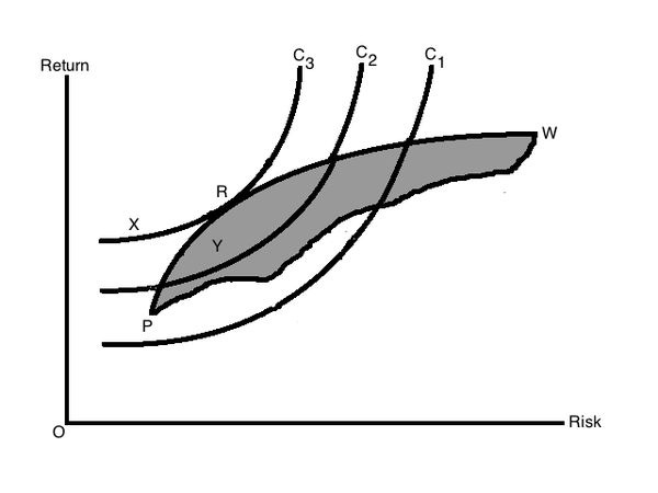
The investor’s optimal portfolio lies at the point of tangency between the efficient frontier and their indifference curve for risk and return.
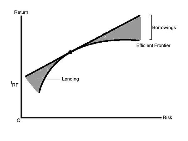
When we add a risk-free asset, the efficient frontier transforms into a straight line, as described by the Mutual Fund Separation Theorem. The Sharpe ratio, defined as:
is geometrically the slope of the line connecting the risk-free rate to the market portfolio. At equilibrium, the risk-free rate is determined by the supply and demand for borrowing and lending.
Under additional (albeit unrealistic) assumptions in the Capital Asset Pricing Model (CAPM), the return of any asset i is purely driven by its exposure to the market and the risk-free rate, as expressed by the Security Market Line (SML):
The core insight of CAPM is that all idiosyncratic (diversifiable) risk should be eliminated in a rational portfolio. Therefore, the only contributor to an asset’s expected return is its systematic (market) risk, measured by beta. If an asset’s price is too low, investors will buy it, pushing its expected return back in line with the SML, and vice versa if it is overpriced.
Single Period Utility Optimization & Constant Absolute Risk Aversion
Under Markowitz/CAPM, we assume that investors care only about the first two moments of portfolio returns (mean and variance). Using λ to represent an investor’s risk aversion, they maximize the mean-variance objective function:
In single-period settings, mean-variance optimization is consistent with utility maximization if the investor’s utility function is quadratic (regardless of return normality), or if returns are normal (regardless of utility shape).
In practice, mean-variance optimization corresponds to maximizing a second-order Taylor approximation of an investor’s true utility function. This means its validity for non-quadratic utility functions depends on the degree to which higher moments (skewness and kurtosis) are significant, which they almost always are in real-world returns. Since normal distributions are completely described by two moments, the approach works neatly under strict normality.
However, in reality, we should focus more on the actual shape of return distributions (i.e., non-normality) rather than strictly on whether an investor’s utility is quadratic.
Quadratic utility functions exhibit two well-known unrealistic properties. First, no matter how small the parameter b, there exists a point beyond which additional wealth actually reduces utility (and for negative b, the investor becomes risk-seeking). Second, quadratic utility implies increasing absolute risk aversion (the negative ratio of the second derivative to the first derivative), meaning that as wealth increases, investors would allocate a lower nominal dollar amount to risky assets, contrary to most empirical evidence.
Multiperiod Portfolio Optimizations & Constant Relative Risk Aversion
For multiperiod portfolio optimizations, assuming return normality (and thus lognormal price dynamics), the target composition of risky assets will remain constant across rebalancing periods only if the investor exhibits constant relative risk aversion (CRRA) utility with respect to wealth. By definition, if an investor's relative risk aversion (RRA) is not constant, they will want to adjust their risk exposure as their wealth changes. Solving the differential equation for CRRA:
we find that the class of CRRA utility functions takes the form:
Applying L’Hôpital’s rule, we see that as γ approaches 1, this utility converges to log utility; as γ approaches 0, it converges to risk-neutral utility. Empirically, estimates of investor relative risk aversion typically fall between 1 and 5. By definition, investors with CRRA utility have portfolio preferences that are independent of their wealth level. This is particularly convenient for portfolio managers modeling these hypothetical investors, as it allows the same portfolio framework to be applied regardless of asset base size.
Kelly Criterion
If I were offered a coin flip with a 1% edge, it might seem reasonable to bet all the cash in my wallet. However, if I were offered the same bet 100 times, it would be unreasonable to go all-in on each flip — even though, by linearity of expectation, that would theoretically maximize expected value in a single shot.
The Kelly Criterion, introduced by John Larry Kelly Jr. in 1956, captures this intuition. As Wikipedia puts it: "The Kelly bet size is found by maximizing the expected logarithm of wealth (i.e., maximizing log utility), which is equivalent to maximizing the expected geometric growth rate of wealth. Assuming expected returns are known, the Kelly criterion leads to higher wealth than any other strategy in the long run (i.e., the theoretical maximum return as the number of bets goes to infinity)."
Heuristic derivations of the Kelly Criterion are fairly straightforward. We start with a unit of wealth and bet a fraction 𝑓 of that wealth on an outcome that occurs with probability 𝑝 and offers odds of 𝑏. The probability of winning is 𝑝, and in that case the resulting wealth is equal to 1 + 𝑓𝑏. The probability of losing is 𝑞 = 1 − 𝑝 and the odds of a negative outcome are 𝑎. In that case the resulting wealth is equal to 1 − 𝑓𝑎. Therefore, the expected geometric growth rate 𝑟 is:
To find the maximum 𝑟 (as a function of f) we can take the logarithm of both sides and differentiate with respect to f. Solving for the f* that gives the maximum growth rate gives us the equation
According to MacLean, Thorp, and Ziemba, the Kelly Criterion has several desirable properties beyond simply maximizing log-wealth. Under broad conditions, it:
Maximizes the median final wealth.
Minimizes the expected time to reach a wealth target.
Asymptotically dominates all other strategies (achieving higher wealth than any other strategy with probability 1 as the number of bets goes to infinity).
Moreover, by the Karush–Kuhn–Tucker conditions, the expected ratio of wealth achieved by any alternative strategy over that achieved by Kelly is ≤ 1 for any horizon — a property known as Competitive Optimality. A direct application of Markov’s Inequality further implies that an opponent cannot outperform the Kelly strategy by a factor of k with probability greater than 1/k.
Continuous Kelly Betting & Mean-Variance Analysis
Consider an investor who wants to create a long-short position using the market portfolio and the risk-free security. Just like in the discrete case of betting, if they wanted to maximize expected wealth, they should theoretically leverage to infinity. However, this has the undesirable consequence of going bankrupt with probability 1. We now consider better options for the investor.
Assume that the market portfolio follows Geometric Brownian Motion with instantaneous drift 𝜇 and volatility σ. Its geometric growth rate is actually lower than 𝜇 since a proportional move down followed by an equivalent move up results in a lower level of wealth. This is a manifestation of the AM–GM inequality.
The actual geometric growth rate of the market portfolio is
where the negative term is often called the “volatility tax” or “volatility drag.” If the investor has CRRA utility with risk aversion parameter γ, then we want to find some proportion x of the risky asset to instantaneously rebalance toward to optimize utility.
In practice, this typically means that a leveraged market portfolio is optimal for long-term capital growth, with the empirical optimal leverage often around 1.75–2.25 over the long run. One may realize that the risk aversion parameter γ of the CRRA utility function coincides with the risk aversion parameter λ in mean-variance optimization.
Optimizing geometric growth rate in continuous time is therefore equivalent to the static single-period optimization of the Markowitz model. It follows that the optimal allocation to the risky asset should be directly proportional to its excess return and inversely proportional to its variance and the investor’s relative risk aversion.
Indeed, where s is the instantaneous Sharpe ratio, we can show rigorously via Itô's lemma that the optimal proportion to allocate toward the risky market portfolio is
It is easy to see that the Kelly strategy is a special case of the optimal solution to the CRRA utility optimization problem. When the risk aversion parameter is 1, the investor has log utility and their investment strategy optimizes the geometric growth rate of wealth. For higher levels of risk aversion, the investor deploys a fractional Kelly strategy and accepts a lower growth rate in exchange for lower risk.
Kelly Betting & Risk Parity
It can also be shown that if two risky assets have the same Sharpe ratios, then the maximal growth rate portfolio is a risk parity portfolio, both in the sense of equal stand-alone risks and equal risk contributions (the former implies the latter).
For the case of more than two assets, if the assets all have the same Sharpe ratio and the correlations are constant, the maximal growth rate allocation will still correspond to a risk parity portfolio. In practice, however, risk parity is more of a marketing term, and there is no fundamental reason why an investor should specifically demand equal risk contributions across assets. Instead, the investor should aim to construct the highest possible Sharpe ratio portfolio and then leverage that portfolio to achieve the desired risk level.
Bringing It Back to Leveraged ETFs
When we connect these theoretical foundations — Markowitz, CAPM, utility maximization, and continuous-time Kelly betting — we see that leveraged index ETFs aren’t necessarily the reckless tools they’re often made out to be. In fact, they can be viewed as a practical implementation of the optimal growth strategy for investors seeking to achieve a specific risk-return profile.
Under this framework, what’s "optimal" leverage is not universal; it depends on each investor’s risk aversion, time horizon, and future income profile. For example, a young investor with stable future earnings (sometimes called "human capital") is effectively underexposed if they invest just 1x in a broad market index. From a lifecycle perspective, they could rationally allocate more aggressively (even beyond 100% equity) to match their total effective wealth. Leveraged index ETFs, in this context, offer a straightforward way to express that higher effective equity exposure without relying on margin accounts or complex derivatives.
When it comes to single-stock leveraged ETFs or similar instruments, their existence also makes theoretical sense. Investors often hold individual stocks to express concentrated bets or personal convictions. Companies themselves do not — and cannot — dynamically lever or de-lever to match every investor’s personal risk appetite. Thus, it becomes the investor’s responsibility to adjust their exposure to meet their own utility and risk preferences.
Disclaimer
The information provided on TheLogbook (the "Substack") is strictly for informational and educational purposes only and should not be considered as investment or financial advice. The author is not a licensed financial advisor or tax professional and is not offering any professional services through this Substack. Investing in financial markets involves substantial risk, including possible loss of principal. Past performance is not indicative of future results. The author makes no representations or warranties about the completeness, accuracy, reliability, suitability, or availability of the information provided.
This Substack may contain links to external websites not affiliated with the author, and the accuracy of information on these sites is not guaranteed. Nothing contained in this Substack constitutes a solicitation, recommendation, endorsement, or offer to buy or sell any securities or other financial instruments. Always seek the advice of a qualified financial advisor before making any investment decisions.