


The square-root formula typically used for the market impact of traded volumes is highly non-trivial; in particular, it means that trading 1/100 of the daily volume moves the price by a 1/10 of its daily volatility, which is a huge amplification. Mathematically, a square-root formula implies that the susceptibility of the market to trades of vanishing size is formally infinite. In this post, we offer intuition as to why this is the case.
Informal Derivation of the Square Root Law
Most derivations of the square root law for market impact build upon some model of market microstructure and then infer the market impact from the model. However, we try to show in this post that the square root law is, in some sense, model agnostic. We will do this by deriving the square root law purely from dimensional analysis (source here). We start first by considering things that could affect market impact
Impact (Δ) This is what we’re trying to measure and will be on the left hand side of our equation; this has units in [%].
Order Quantity (Q) A bigger order must have a bigger impact than a smaller order, else there is arbitrage; this has units in [shares].
Average Volume (V) Intuition suggests that all else held equal, it is easier to trade something that trades a lot with less impact than to trade something that doesn’t trade as much. From the market maker’s perspective, it is easier to externalize risk when trade volume is high; this has units [shares]/[time].
Volatility (σ) Again, intuition suggests that a security which moves around a lot is going to be tougher to trade. Assuming non-arbitrage, the stock’s returns over time are iid, and therefore volatility has units [%]*[t]^(1/2).
Bid-Ask Spread (s) this by definition impacts every trade, even ones too small to otherwise move the price, this has units in [%].
On the LHS we have units of %, so our right side must also have units of percent. Spread also has units of % so this can be added or subtracted; however, all other units must be multiplied or divided (you can have a meter/second, but not a meter + second). In other words, for the equation to make sense, we must have
For the dimensions to match up, we need to have
a = -b to get rid of the [shares] unit
b = -c/2 to get rid of the [time] unit
c = 1 since it is the only [%] unit
k1 = 1 since when Q = 1 we pay the spread once
k2 = free parameter to be measured empirically
Regarding a, b, and c, this is a linear system of three equations in three variables, and it can be solved easily to get us the square root formula
To see if the square root law holds up empirically, we can graph the trade impact and the volume together on a log-log plot and run a regression to see if the slope is indeed around 1/2 (in general, if we know something to be in the form a = b^x and we want to determine x, we can graph a against b in a log-log plot to run a linear regression).
In the figure below we see the impact of orders for trades on US futures markets in the period June 2007 to December 2010. The Log-log plot is that of the volatility-adjusted price impact vs the ratio Q/V. Source here.
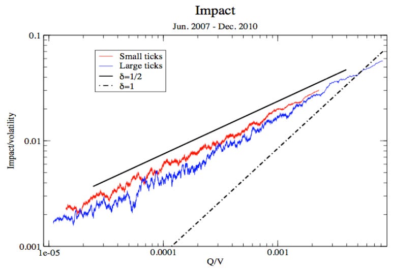
We see that the square-root market impact formula is verified empirically for orders with a range of sizes spanning two to three orders of magnitude. It is interesting to note that time does not appear in this formula; as such, it would suggest that the rate of trade and the method of execution both have negligible effect on the impact of the trade; this is highly unintuitive and ultimately false; but it is generally true that the effects of slower / faster trading and more / less sophisticated execution are secondary when compared to the volume, volatility, and trade size.
The Nature of Liquidity and Volatility
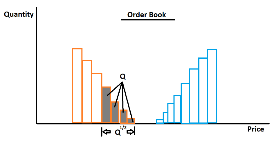
The square root law has a geometric interpretation that arises according to the nature of the limit order book near the boundary between buying and selling. In particular, let us assume that the limit order book represents the supply/demand curve for an asset at values differing from its current price. This function is surely differentiable (forgive my assumptions) and as such is locally linear near the intersection of supply and demand. As such, we can assume that the order book is locally linear near the mid-price, and for a slope of λ on the order book the order will have an impact of
This is the same formula as previously derived, with
Rearranged, this shows us what volatility is from a microstructure perspective
I.e. a security’s variance is proportional to the ratio between the arrival rate of trades (liquidity demand) to the steepness of the order book (liquidity supply). This should be intuitive since if a lot of trades arrive very quickly, or if the order book is shallow, then a security will be volatile, and vice versa. The relationship between liquidity and volatility is also made clear in that specifically, liquidity has an inverse relationship with volatility; an increase in liquidity can help dampen volatility, but increased volatility can also reduce liquidity.
The geometric picture also provides intuition as to why smaller trades appear to move prices disproportionately more than they should (1/100 of the daily volume moves the price by a 1/10 of its daily volatility); specifically, by definition liquidity vanishes at crossing price, and if supply and demand curves are locally linear, then the square root law emerges naturally. In other words, if people wanted to trade near the mid-price, then they would have already traded, and as such there won’t be much liquidity there.
Viewing volatility as a function of both liquidity demand (trade arrival rate) and liquidity supply (order book steepness) offers a powerful unifying principle for understanding a range of market phenomena that often seem unrelated at first glance.
For example, it offers a natural lens through which to understand why earnings or event volatility can be correlated with realized volatility prior to earnings even though the amount of information released during an earnings event is largely fixed and independent of prior price action. If we take volatility to reflect not just the presence of information but also market capacity to absorb that information, then the connection becomes clearer i.e. earnings volatility isn't just about what’s in the report but also about how efficiently the market can process it.
When diffusive volatility is high, we can infer that liquidity demand is higher than typical liquidity supply; even in the absence of a fundamental catalyst, prices move more because each trade carries more price impact. In this environment, any scheduled information release, like earnings, will be absorbed less smoothly, amplifying its potential to move prices. Thus, the option market may bid up earnings vol because the market is already fragile and reactive. Conversely, when volatility is low, markets are calm, order books are thick, and trades are absorbed without much movement, the same earnings information can be expected to cause more muted price reactions, leading to cheaper pricing of earnings vol.
Put differently, while the total information content of earnings doesn't change, its market impact does, depending on how robust the market’s liquidity infrastructure is at that time. Since both event volatility and diffusive volatility emerge from the same microstructural roots—namely, how much trading pressure exists and how deep the liquidity is—it makes sense that the two should be correlated.
The same principle clarifies volatility clustering. In periods of elevated trade activity or thinning liquidity—perhaps due to uncertainty, positioning imbalances, or exogenous shocks—price impact per trade rises. This higher impact reduces market-maker willingness to post size (they are more exposed to adverse selection), which further decreases book steepness, raising volatility even more. This creates a feedback loop where high volatility begets low liquidity, which begets more volatility. This is not a function of information arrival alone but of how much stress is placed on the liquidity infrastructure.
Consider also, for instance, the volatility that arises from passive flows. While ETFs and index funds rebalance systematically and without discretion, the market’s ability to absorb those trades can be unstable. During a quarterly index rebalance, if hedge funds and arbitrageurs that typically intermediate these flows are sidelined—whether due to poor performance, risk constraints, or outright blow-ups—the liquidity supply that would normally meet the surge in demand disappears. This means that even a predictable, mechanical flow can cause outsized price movements when the capacity to absorb it has vanished. The volatility, in this case, doesn't come from new information about the constituents, but from the collapse of liquidity that would usually keep prices stable.
Even phenomena like correlation spikes during selloffs can be understood through this lens. It’s not that information suddenly becomes shared across assets; it’s that liquidity providers withdraw in tandem across names when volatility rises. As trade arrival rates spike and books thin, the marginal impact of trades rises everywhere, mechanically increasing observed correlation. This isn't necessarily fundamental—it’s microstructural.
In all these cases, volatility is less about what we know or don’t know, and more about how much stress the market is under in its ability to absorb trading pressure. Liquidity is not just a background condition but rather it is the very medium through which information is expressed in prices.
Summary
The square-root law, derived through dimensional analysis, shows that market impact scales with the square root of trade size relative to average volume, showing that price impact remains significant even for small trades. Empirical studies confirm this relationship across multiple markets. A microstructural perspective links market impact to liquidity and volatility, revealing that a security's volatility depends on the interplay between trade arrival rates and order book depth. The geometric interpretation of supply and demand curves near the mid-price helps clarify why price moves disproportionately to trade size, as liquidity is naturally sparse in this region.
Disclaimer
The information provided on TheLogbook (the "Substack") is strictly for informational and educational purposes only and should not be considered as investment or financial advice. The author is not a licensed financial advisor or tax professional and is not offering any professional services through this Substack. Investing in financial markets involves substantial risk, including possible loss of principal. Past performance is not indicative of future results. The author makes no representations or warranties about the completeness, accuracy, reliability, suitability, or availability of the information provided.
This Substack may contain links to external websites not affiliated with the author, and the accuracy of information on these sites is not guaranteed. Nothing contained in this Substack constitutes a solicitation, recommendation, endorsement, or offer to buy or sell any securities or other financial instruments. Always seek the advice of a qualified financial advisor before making any investment decisions.