Options Implied Distributions are NOT Real-World Distributions

From The Logbook. The original article is reproduced in full, with minor grammar corrections; references to market conditions reflect the context in which it was written.

There is sometimes a misunderstanding, even among practitioners, that option prices reflect the market’s view of the distribution of an asset’s price at expiry. This emerges out of a serious misunderstanding of the difference between the risk-neutral measure used to price derivatives in complete markets and the real-world measure that determines the actual distribution of asset prices. We try not to dive too deep into the math here, proof outlines and statements of the main theorems are usually enough, but a working knowledge of probability and option theory (academic, not practical) is helpful.

Introduction

This post is dense. The argument moves through the following steps:

How “implied probabilities” are constructed: tight butterfly spreads + an interpolated volatility surface yield a risk-neutral density.
Why the drift disappears: the delta-hedging argument removes μ from the option-pricing PDE, leaving only r.
Existence and uniqueness of ℚ: Fundamental Theorem of Asset Pricing and the Law of One Price tie no-arbitrage and completeness to the risk-neutral measure.
Construction via Feynman–Kac and Girsanov: change of measure makes the bridge between ℙ and ℚ explicit and is consistent with equilibrium models.
The stochastic discount factor (SDF): the object that takes us back and forth between ℙ and ℚ is also the intertemporal marginal rate of substitution.
Why ℚ deflates the price distribution: exponential compounding at μ>r inflates absolute deviations under ℙ, so ℚ-probabilities exaggerate downside.
Trading implications: call-buys and put-sales can be positive-EV under ℙ, but under CAPM equilibrium they are inferior leveraged exposure to the market.
When implied views align with reality: short maturities, earnings, and incomplete markets.

Options-Implied Probabilities (Definitions)

Exposure to a specific range of stock-price outcomes can be acquired with a butterfly spread (long 1 low-strike call, short 2 calls at a higher strike, long 1 call at an even higher strike). The “probability” of the stock ending in that range is then computed as the cost of the butterfly divided by the payoff if the stock lands in the range.

To extrapolate a full distribution, first interpolate an implied-volatility surface from observable discrete strikes, then price a sequence of theoretical calls at arbitrarily fine strikes from the interpolated surface. Tight overlapping butterflies built from these calls give probabilities for arbitrarily narrow ranges; dividing each butterfly’s cost by its payoff (and discounting) gives the implied density.

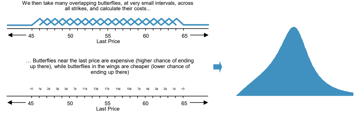
The remainder of this post argues that using options-implied probabilities to estimate future stock prices yields a distribution with expected returns and perceived risk meaningfully lower than the market’s actual expectations.

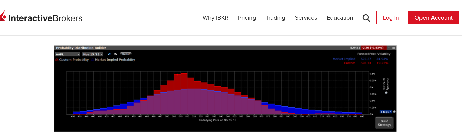
For brokerage firms, presenting the options market as underpricing expected return can attract retail flow and the fees that come with it. IBKR’s Probability Lab, for example, lets retail traders view the “market-implied distribution” and identify “optimal” trades against their own view:

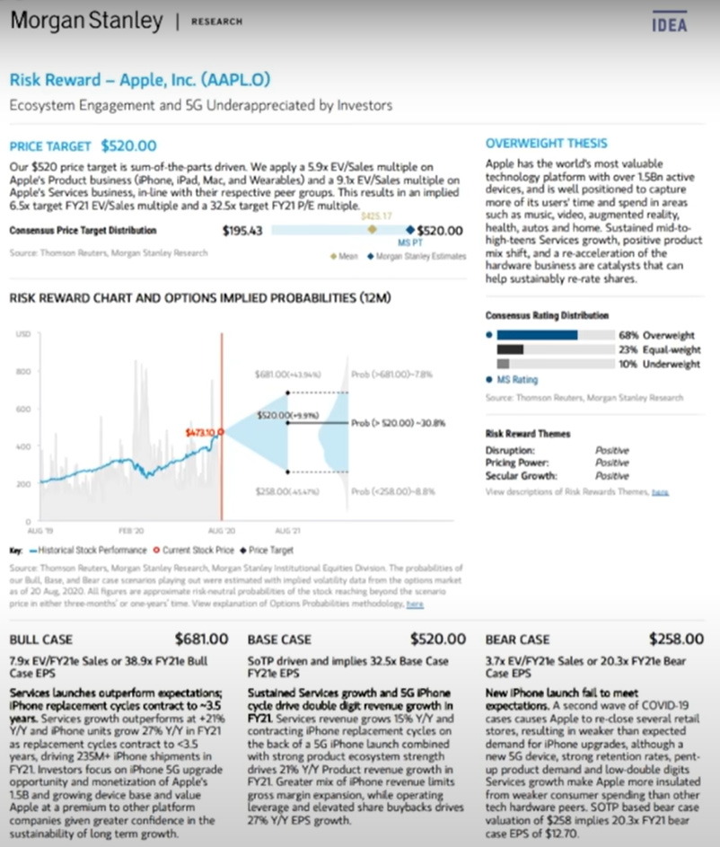
Sales-and-trading desks face a similar incentive: presenting investments as less risky than they really are encourages clients to size up or stretch into asset classes they would otherwise avoid. Consider this Morgan Stanley research excerpt on AAPL:

To say with rigor why these presentations are misleading, we have to first fix some terminology. The point of the post is that the risk-neutral measure differs from the physical market measure, so we begin by defining what a “measure” is.

What is a Probability Measure? (Definitions)

The Wikipedia definition is unhelpful: a probability measure is “a real-valued function defined on a set of events in a σ-algebra that satisfies measure properties.” Here is the same idea unwrapped on the example of a fair coin. A probability space consists of:

A sample space X, the set of all possible outcomes.
A collection of events Σ, which are subsets of X.
A function μ, the probability measure, that assigns each event in Σ a non-negative real number.

In the case of flipping a fair coin, we have

X=\{H,T\}

\Sigma=\{\varnothing,\{H\},\{T\},X\}

\mu(\varnothing)=0, \ \ \mu(\{H\})=\mu(\{T\})=\frac{1}{2},\ \ \mu(X)=1

All of this to say that when I flip a coin, I have a 0 percent chance of flipping nothing, a 50 percent chance of flipping heads, a 50 percent chance of flipping tails, and a 100 percent chance of flipping something. This is all very intuitive.

There are certain natural requirements that Σ and μ must satisfy. For example, it is natural to require that ∅ and X are elements of Σ, that μ(∅) = 0, and that μ(X) = 1 (i.e. when performing an experiment, the probability that no outcome occurs is 0, while the probability that some outcome occurs is 1). There are other requirements of μ which make it a (finite) measure, but in essence a measure is simply a function that assigns to each event in Σ a nonnegative real number.

Similarly, it is natural that there are some requirements we think Σ should have in relation to μ (note that the prior constraints on μ were independent of Σ). For example, if E ∈ Σ is an event, then μ(Eᶜ) + μ(E) = 1 (i.e. when performing an experiment, the probability that event E occurs or doesn’t occur must be 1). There are, of course, other requirements of Σ which make it a σ-algebra, but in essence a σ-algebra is just a set of events that satisfies very reasonable logical constraints.

Market Measures: ℙ and ℚ (Definitions)

In a market context the sample space encodes possible outcomes of financial variables and events are subsets we care about (e.g., “the stock closes above K at time T”). Two probability measures are central to the rest of the post:

Physical Measure (ℙ). The probability measure that reflects actual investor expectations and behaviors, accounting for risk preferences and all other market forces. ℙ-probabilities forecast actual outcomes but are unobservable; we never see a probability label written on the market.

Risk-Neutral Measure (ℚ). The probability measure under which all investors are as if risk-neutral: assets are expected to drift at the risk-free rate, and any contingent claim’s price equals the discounted expected payoff under ℚ. This is a mathematical construct, not a forecast, and it is what option prices imply.

The TLDR is that ℚ adjusts ℙ so the expected discounted return of every asset becomes the risk-free rate (i.e., everything earns exactly the risk-free rate in expectation). Equivalently, ℚ is what you get when you fold investors’ risk premia into the probabilities themselves rather than into a separate discount rate. The transformation is concrete and we will write it down explicitly in the later section.

Drift Disappears in Derivative Pricing (Proof)

Assume the stock price St follows a Geometric Brownian Motion under ℙ:

\frac{dS_t}{S_t} = \mu dt + \sigma dW_t^{\mathbb{P}}

where μ is the expected return and σ the annualized volatility of log-returns. Consider any contingent claim Vt=V(t,St) that pays ϕ(ST) at time T (a generic European option). Form the self-financing portfolio

\Pi_t = V_t - \alpha S_t

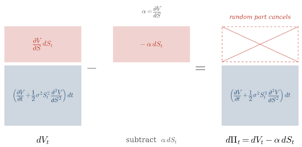
By Itô’s lemma and the self-financing property,

\begin{align} d\Pi_t &= dV_t - \alpha dS_t \\ &= \left( \frac{\partial V}{\partial t} + \frac{1}{2} \sigma^2 S_t^2 \frac{\partial^2 V}{\partial S^2}\right) dt + \left( \frac{\partial V}{\partial S} - \alpha \right) dS_t\\ \end{align}

Black, Scholes, and Merton’s original argument was that if we continuously rebalance so that α=∂V/∂S (delta-hedging), the random dSt term vanishes and Πt drifts deterministically. By no-arbitrage that drift must be the risk-free rate. So

\begin{align} &d\Pi_t = \Pi_t r dt \\ \iff& \left( \frac{\partial V}{\partial t} + \frac{1}{2} \sigma^2 S_t^2 \frac{\partial^2 V}{\partial S^2} \sigma^2 \right) dt = \left( V_t - \frac{\partial V}{\partial S} S_t \right) r dt \\ \iff& \frac{\partial V}{\partial t}(t,S) + r S \frac{\partial V}{\partial S}(t,S) + \frac{1}{2} \sigma^2 S^2 \frac{\partial^2 V}{\partial S^2}(t,S) - rV(t,S) = 0 \end{align}

which is of course the Black-Scholes equation. Notice what is not in it: μ. The real-world drift dropped out the moment we delta-hedged. The cost of replicating the option no longer depends on whether the stock is expected to return 4% or 40%. only on the dispersion σ and the cost of carry r.

Existence and Uniqueness of ℚ (Statement of Core Results)

The delta-hedge argument shows that an option (or any contingent claim) can be manufactured by a replication argument, static for linear contracts, dynamic for others, and that its value satisfies the Black–Scholes PDE under the assumptions of no arbitrage, market completeness, continuous trading, and no frictions. Since all such replicating portfolios grow at the risk-free rate, the option can equivalently be priced as if the underlying drifted at r; that is the idea of “risk-neutral” valuation

Another simple concrete instance: a forward contract. Buy the stock now and sell the forward; the net position is risk-free, so by absence of arbitrage the forward price equals the spot grown at r. The same valuation comes from assuming the stock drifts at r under ℚ. The fact that a 10-year SPX forward trades at the risk-free forward rate does not mean anyone expects U.S. large-caps to return only r for the next decade. It is a feature of the measure used, not a forecast.

Two core results in financial economics formalizes the above intuition

Fundamental Theorem of Asset Pricing: The condition of no-arbitrage is equivalent to the existence of a risk-neutral measure.
Law of One Price: Market completeness is equivalent to the uniqueness of the risk-neutral measure.

Together these say that in a complete, arbitrage-free market there is one and only one measure ℚ under which discounted asset prices are martingales, and pricing under ℚ is equivalent to pricing by replication. This is why mathematical finance separates into two regimes: ℙ for risk and portfolio management, ℚ for derivatives pricing. The split exists because derivative values must grow at r by replication, while fundamental assets, the things that can’t be manufactured from cheaper pieces, require a risk premium. A full proof is long; but below we give an outline that is useful for intuition.

Construction of ℚ Under Black-Scholes (Proof)

The Black–Scholes PDE is parabolic. The Feynman–Kac formula establishes the link between parabolic PDEs and stochastic processes: the PDE describes the flow of a time-dependent probability density, and a related stochastic process describes individual realizations, random walks with drift, whose distribution, run many times, reconstructs the density. The formal statement is that for the PDE

{\frac {\partial }{\partial t}}u(x,t)+\mu (x,t){\frac {\partial }{\partial x}}u(x,t)+{\tfrac {1}{2}}\sigma ^{2}(x,t){\frac {\partial ^{2}}{\partial x^{2}}}u(x,t)-V(x,t)u(x,t)+f(x,t)=0

defined for x∈ℝ and t∈[0,T] with terminal condition u(x,T)=ψ(x), the solution admits the probabilistic representation

u(x,t)=E^{Q}\left[e^{-\int _{t}^{T}V(X_{\tau },\tau )\,\mathrm {d} \tau }\psi (X_{T})+\int _{t}^{T}e^{-\int _{t}^{\tau }V(X_{s},s)\,\mathrm {d} s}f(X_{\tau },\tau )\,\mathrm {d} \tau \,{\Bigg |}\,X_{t}=x\right]

where X is the Itô process

\mathrm {d} X_{t}=\mu (X_{t},t)\,\mathrm {d} t+\sigma (X_{t},t)\,\mathrm {d} W_{t}^{Q}

and Wℚ is a Brownian motion under ℚ. (The physics interpretation is that a particle diffuses, accumulates running cost f, has a final cost ψ, and decays at rate V; u(x,t) is its expected cost-to-go.) Apply this directly to Black–Scholes: the PDE is matched by setting the discount V≡r and forcing f≡0, and the terminal condition is ϕ(ST). The representation gives

V_0 = E^\mathbb{Q}[ e^{-rT} \phi(S_T) \vert \mathcal{F}_0 ]

with St evolving as

\frac{dS_t}{S_t} = r dt + \sigma dW_t^{\mathbb{Q}}

The drift under ℚ is exactly r, which is what we wanted to show.

Consistency of Black-Scholes with General Equilibrium (Proof)

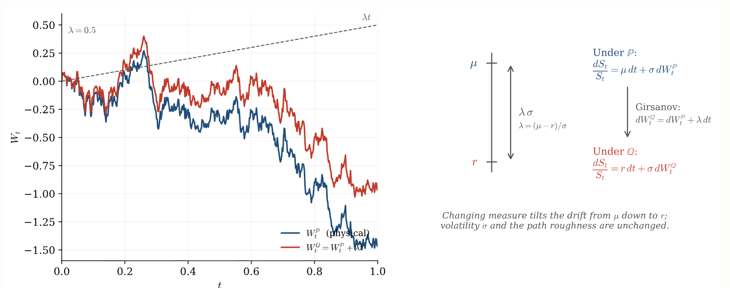
Feynman–Kac gives the answer but feels like a magic trick. Zooming in on the change of measure makes the bridge between ℙ and ℚ explicit. Define λ as the Sharpe ratio of the stock, the excess return per unit of volatility. Then under ℙ,

\frac{dS_t}{S_t} = r dt + \sigma (dW_t^{\mathbb{P}} + \lambda dt)

Girsanov’s theorem says that there is a measure ℚ, equivalent to ℙ, under which dWtℚ:=dWtℙ+λdt is a Brownian motion. Substituting recovers the ℚ-dynamics from the previous section. Manipulating the Radon–Nikodym derivative gives

V_0 = E^{\mathbb{Q}} \left[ e^{-rT} \phi(S_T) \vert \mathcal{F}_0 \right] = E^{\mathbb{P}} \left[ e^{-\left(r+\frac{\lambda^2}{2}+\frac{\lambda}{T} W_T^{\mathbb{P}}\right)T} \phi(S_T) \vert \mathcal{F}_0 \right]

This gives two readings of the same option price:

Under ℚ: discount cash flows at the risk-free rate.
Under ℙ: discount cash flows at a stochastic rate that bakes in the market price of risk λ (which depends on μ).

In short, an option should cost the same to a hedger who delta-hedges (and earns r) as to a speculator who holds it outright (and is exposed to a higher expected return but also higher risk), provided both are pricing rationally.

Forward on the market portfolio is the cleanest example. Replication yields the risk-free rate (which lies on the Security Market Line, satisfying CAPM). Buying the forward outright gives leveraged exposure to the market portfolio (also on the SML). The expected return is higher in the second case but is discounted at a correspondingly higher rate, so the present value is still the same.

Under the physical measure, prices depend on risk: investors demand higher returns for higher risk, so today’s price of a risky payoff lies below its expected value, compensating the bearer. In a complete arbitrage-free market every derivative can be replicated by dynamic hedging, leading to the Black–Scholes PDE governing all contingent-claim prices; for certain boundary conditions we get closed-form solutions, though not in every case.

There is a unique measure ℚ, equivalent to ℙ, under which all investors behave as if risk-neutral; switching to ℚ embeds the risk premia into probabilities. Taking expectations under ℚ gives the same answer as solving Black–Scholes.

The Stochastic Discount Factor (Interpretation)

We can now answer: what, formally, takes us from ℙ to ℚ? From above, with a particular risk premium λ assumed, the expectation under ℚ equals the expectation under ℙ discounted by a stochastic factor:

V_0 = E^{\mathbb{Q}} \left[ e^{-rT} \phi(S_T) \vert \mathcal{F}_0 \right] = E^{\mathbb{P}} \left[ e^{-\left(r+\frac{\lambda^2}{2}+\frac{\lambda}{T} W_T^{\mathbb{P}}\right)T} \phi(S_T) \vert \mathcal{F}_0 \right]

If Black–Scholes assumptions hold, estimating real-world probabilities is straightforward, calibrate μ and σ to a time series. The general case is more interesting. Under mild regularity conditions,

V_0 = E^{\mathbb{Q}} \left[ \frac{V_T}{B_T} \vert \mathcal{F}_0 \right] = E^{\mathbb{P}} \left[ \frac{V_T}{B_T} f \vert \mathcal{F}_0 \right], \ \ \ \ \ f = \left. \frac{d\mathbb{Q}}{d\mathbb{P}} \right\vert_{\mathcal{F}_T}

where BT is the money-market numeraire. Define the risk-free discount factor and the Stochastic Discount Factor:

DF (0,T):=1/B_T, \ \ \ \ \ SDF (0,T):=f/B_T

Then in general,

V_0 = E^{\mathbb{Q}} \left[ DF (0,T) V_T \vert \mathcal{F}_0 \right] = E^{\mathbb{P}} \left[ SDF (0,T) V_T \vert \mathcal{F}_0 \right]

Closed-form f is special to Black–Scholes. For incomplete models, jumps, stochastic volatility, etc. there is no clean expression.m We have just seen that an SDF emerges from the existence of a risk-neutral measure. The converse is more enlightening: ℚ emerges from the existence of an SDF. Consider a state space:

Let X be a random variable denoting a risky cash flow next period.
Let f(X) be a pricing function: today’s price for a risky cash flow.

Linearity of f is an obviously desirable property. If f is linear, there exists a stochastic discount factor M with

f(X) = \operatorname{E}^\mathbb{P}[MX]

In a discrete probability space with n outcomes, this becomes

f(X) = \sum_i p_i m_i x_i

The M is inconvenient. Define

q_i = \frac{p_i m_i}{\sum_j p_j m_j}

Then ∑iqi=1, so ℚ is itself a probability measure. The risk-free rate satisfies 1=∑ipimi(1+rf), hence ∑ipimi=1/(1+rf). Putting it together,

\operatorname{E}^\mathbb{P}[MX] = \sum_i p_i m_i x_i = \frac{1}{1+r_f} \sum_i q_i x_i = \frac{1}{1+r_f} \operatorname{E}^\mathbb{Q}[X]

again showing that there are two equivalent ways to price (without Black-Scholes)

The physical measure ℙ together with the SDF M.
A tilted measure ℚ together with risk-neutral discounting.

Each state i can have a different state price; risk-neutral pricing is a convenient packaging that absorbs state prices into a tilted measure ℚ proportional to p⋅m. What takes us back and forth between ℙ and ℚ is the stochastic discount factor M.

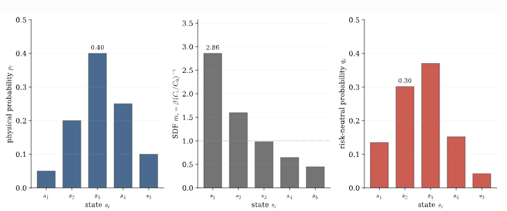
So despite its name, the risk-neutral measure is affected by risk aversion. The physical measure represents true probabilities; the risk-neutral measure embeds the risk premia by re-weighting via the SDF (mathematically, by Girsanov).

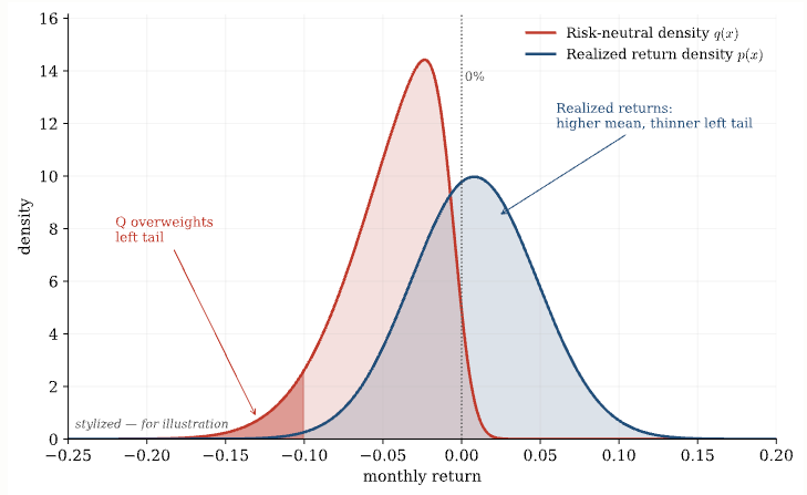
The implications for interpretation are non-trivial: in a risk-neutral world, the probabilities for different outcomes are tilted to make investors act as if they don’t require risk compensation, which means downside risks are exaggerated relative to the real-world probabilities. The risk-neutral probabilities backed out of option prices should not be naively read as the actual probabilities investors assign.

This is a partial explanation for the volatility skew: out-of-the-money puts trade at higher implied volatility than equidistant out-of-the-money calls because investors care more about losses than equivalent gains, so the SDF M puts more weight on bad states, and ℚ inherits that tilt.

Intertemporal Marginal Rate of Substitution (Interpretation)

What should the SDF be? Financial economists have spent decades on this question with limited success. Formally, if a representative agent has additively-separable utility over consumption,

U(C) = \sum_{t=0} \beta^t u(C_t)

then the SDF is the intertemporal marginal rate of substitution

M_{t+1} = \beta \frac{u'(C_{t+1})}{u'(C_t)}

In plain words, the SDF is a state- and time-dependent random variable whose value tells you the right discount for cash flows in that state. It is stochastic because the state of the world is random. We typically think of states as consumption levels, so an asset that pays well when consumption is high (a cyclical asset, like stocks) is less valuable than one that pays well when consumption is low. We would prefer payoffs that arrive when we are poor, not when we are rich.

Stocks are naturally the cyclical kind: salaries rise with the economy, so do equity returns. Because people have decreasing marginal utility in consumption, i.e., that they are risk-averse, equity cash flows are discounted at a higher rate than risk-free ones, and earn the equity risk premium.

Hansen and Jagannathan gave the canonical bound on how much volatility any SDF must carry to be consistent with observed Sharpe ratios; consumption-based SDFs notoriously fail this bound, forming the equity risk premium puzzle.

Theory also predicts the SDF M(R) should be monotonically decreasing in the gross return R=ST/S0, i.e. better states get less weight. Empirically that’s not what shows up in S&P options. Jackwerth documents a non-monotonic empirical kernel with a hump near at-the-money, directly contradicting the representative-agent CRRA prediction. This is forms the pricing-kernel puzzle.

ℚ Deflates the Price Distribution (Implications)

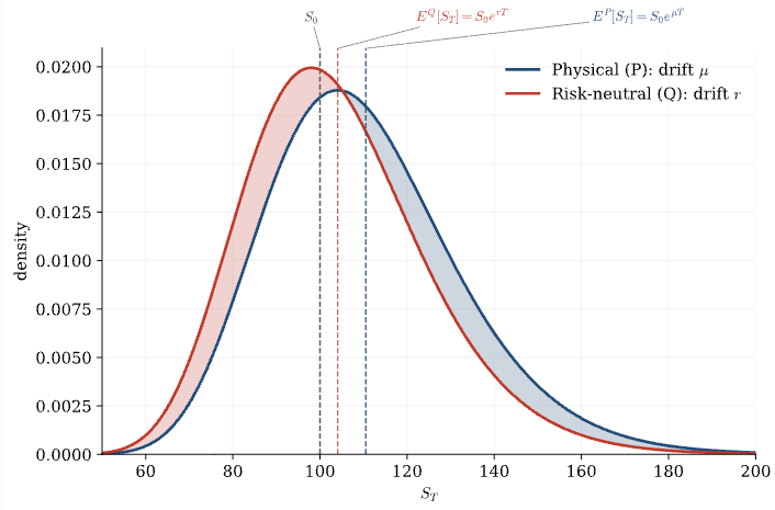
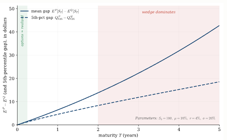
The expected growth rate μ under ℙ typically includes a risk premium and exceeds r. Because returns compound exponentially, the gap shows up not just in expected values but in the scale of price deviations. Under GBM with the same volatility:

E^P[S_T] = S_0 e^{\mu T}, \ \ \ \ \ \text{Var}^P(S_T) = S_0^2 e^{2\mu T} (e^{\sigma^2 T} - 1)

E^Q[S_T] = S_0 e^{r T}, \ \ \ \ \ \text{Var}^Q(S_T) = S_0^2 e^{2r T} (e^{\sigma^2 T} - 1)

Both the mean and the absolute price dispersion scale exponentially with the drift. Constant return volatility is exponentially-growing price volatility, and the price level is higher when μ is higher, so the absolute dollar movements under ℙ are bigger than under ℚ. Over multi-year horizons the gap is non-trivial; this is the mechanical reason a 5-year option-implied distribution looks more conservative than realized return.

Trading Options can be +EV (Implications)

In the post Arbitrage is a Hall of Mirrors, Kris Abdelmessih discusses how arbitrage-free pricing in options can produce trades that look great to a directional investor.

The example provided is based on closing Tesla (TSLA) option prices as of January 28, 2025, for options expiring on January 15, 2027. With TSLA's stock price around $396.65 at the time (rounded to $400 for simplicity) the strategy entails buying a 25% out-of-the-money put at the 300 strike for about $56, and selling a 25% out-of-the-money call at the 500 strike for about $108. This setup allows the investor to collect about $52, or roughly 13% in premium; i.e. if TSLA drops $100 in 2 years, the investor is stopped out at $300 but nets only a $48 loss due to the $52 premium collected. Conversely, if TSLA climbs to $500, the investor would gain $100 on the stock and keep the $52 premium, totaling a 38% gain.

You can stay long the stock, but you get paid 3× as much on a +$100 move as you lose on a −$100 move. It looks like free money, and in a sense, it is. Paraphrasing Kris:

Because risk-neutral probabilities don’t need to reflect real-world probabilities, this can produce a difference of opinion in which the arbitrageur and the speculator are happy to trade with each other. The arbitrageur has a short time horizon, bounded by the riskless arbitrage; the speculator, while not arbitraging, believes they are being overpaid to warehouse risk.

The most prominent live example is Warren Buffett selling deep-OTM index puts during the financial crisis. He took the view that markets would rise over the long run, the options would expire worthless, and he would keep the premium. This is positive expectancy, and it is effectively payment for warehousing equity and volatility risk premium.

Options Aren’t the Best Trade (Implications)

Should you put on the TSLA collar or sell index puts? Maybe, but first ask what the trade actually does and whether better alternatives exist. In some sense, both the TSLA collar and Buffett’s put-selling are ways to collect the equity risk premium. (Unless the options are mispriced, in which case the strategies are simply good trades.)

Under a general-equilibrium model like CAPM, these strategies can be less efficient in mean-variance terms than leveraged exposure to the market portfolio. The TSLA collar only profits when TSLA goes up, and unless TSLA has alpha over the market, its weight in your portfolio should be proportional to its weight in the market portfolio, the strategy is long TSLA delta, hence long beta, and if beta is the only driver of returns then the market portfolio is the best way to take long-beta exposure.

Under CAPM equilibrium a leveraged position in the market portfolio is the optimal risk-return trade-off because of diversification: idiosyncratic TSLA risk is diversifiable, and leveraging the market lets you scale the equity risk premium up without taking unsystematic risk along for the ride.

A slightly different argument applies to put-selling. Under constant relative risk aversion (CRRA), the optimal leverage ratio is constant in wealth. But an index put has spot-dependent delta (i.e., non-zero gamma) and so cannot be a CRRA-rational holding unless it is dynamically hedged, at which point it is just risk-free.

So both the TSLA collar and the index put can be positive-expectancy for the speculator yet not the most efficient trade available (unless the options are mispriced or utility is not CRRA). The market’s risk preferences are already priced in.

When ℙ = ℚ (Counterpoint)

Option-implied distributions can closely match the physical measure, just not over the 1- to 2-year horizon where the most “juicy” trades with LEAPS show up. Over short durations, and particularly in incomplete markets, overnight earnings announcements, idiosyncratic catalyst windows, option prices give a reasonable picture of the expected distribution of underlying prices.

The compounding gap between μ and r has not had time to inflate, the SDF tilt is small relative to the noise, and uniqueness of ℚ may not even hold in incomplete markets, which removes some of the mathematical force of the wedge.

Takeaways

The distinction between risk-neutral and physical measures is a cornerstone of financial mathematics, and it has been well-understood for over fifty years. Practical use of these concepts is often misunderstood or misrepresented even among practitioners. Platforms catering to retail and institutional investors sometimes blur the distinction and this can mislead users into bad decisions.

Education platforms simplify; in simplifying, they often fail to convey the difference between risk-neutral pricing (a theoretical risk-free world used to value derivatives by replication) and the physical measure (the actual probabilities of outcomes, accounting for risk preferences). The result is investors reading option-implied distributions as forecasts.

The pervasive issue may not be entirely about inducing trading for fees. It is plausibly more often the result of ignorance or incomplete understanding among content creators rather than deliberate misdirection. Hanlon’s razor may apply.

Disclaimer

The information provided on TheLogbook (the "Substack") is strictly for informational and educational purposes only and should not be considered as investment or financial advice. The author is not a licensed financial advisor or tax professional and is not offering any professional services through this Substack. Investing in financial markets involves substantial risk, including possible loss of principal. Past performance is not indicative of future results. The author makes no representations or warranties about the completeness, accuracy, reliability, suitability, or availability of the information provided.

This Substack may contain links to external websites not affiliated with the author, and the accuracy of information on these sites is not guaranteed. Nothing contained in this Substack constitutes a solicitation, recommendation, endorsement, or offer to buy or sell any securities or other financial instruments. Always seek the advice of a qualified financial advisor before making any investment decisions.