Is Your Sharpe Lying? | Freeport Markets

From The Logbook. The original article is reproduced in full, with minor grammar corrections; references to market conditions reflect the context in which it was written.

We evaluate the probability that an estimated Sharpe ratio exceeds a given threshold. This allows us to (1) establish the track record length needed for rejecting the hypothesis that a measured Sharpe ratio is below a certain threshold with a given confidence level (2) model the trade-off between track record length and undesirable statistical features (e.g., negative skewness & positive excess kurtosis) (3) optimize a portfolio under non-Normal, leveraged returns while incorporating the uncertainty derived from track record length. This post is based on the paper The Sharpe Ratio Efficient Frontier by Bailey and López de Prado.

The Sharpe Ratio

The Sharpe Ratio is a measure of risk-adjusted returns, defined as the ratio of the excess return of an asset or strategy to its standard deviation. Mathematically, it is

S = \mu / \sigma

where μ is the mean excess return (over a risk-free rate / cost of financing) and σ is the standard deviation of returns. The Sharpe Ratio has a direct link to a t-statistic, which is a measure of whether an observed effect, such as excess returns, is significantly different from the null hypothesis (e.g., zero); in particular, it quantifies how many standard errors the sample mean is away from the mean under the null hypothesis. For a sample of n independent returns (assuming daily), the t-statistic’s relationship with the Sharpe ratio can be expressed as

t = S\sqrt{n}

In other words, the Sharpe ratio can be interpreted as an annualized t-statistic. However, this link becomes more nuanced because the Sharpe Ratio is not just a test of whether returns are nonzero—it is also a measure of performance, capturing the balance between excess return and risk. While the t-statistic for a Sharpe Ratio tests whether the observed risk-adjusted returns are statistically significant (i.e., unlikely to be due to chance), the Sharpe Ratio itself is also used to gauge how good the strategy is in terms of delivering returns per unit of risk.

This dual role complicates interpretation. A strategy could have a statistically significant Sharpe, indicating the returns are reliably nonzero, and indeed have positive excess returns, but still realized a much lower Sharpe than anticipated. When allocating capital across multiple strategies with different Sharpe Ratios, the challenge is not merely deciding whether to invest or not in a single strategy, but determining the optimal allocation of resources among strategies.

The Sharpe Ratio, as a measure of risk-adjusted performance, is often used to guide these decisions. Things become problematic when Sharpe Ratios are inflated due to sampling variability / overfitting, leading to overly optimistic decisions. While a strategy with a high Sharpe might show statistically significant positive returns, the point estimate does not capture the uncertainty in its measurement. To make better allocation decisions, one must consider the confidence intervals or the potential error in the Sharpe Ratio estimate, penalizing strategies with higher uncertainty. Without accounting for this variability, capital could be disproportionately allocated to strategies with inflated Sharpe Ratios, which might underperform in practice, while more robust but understated strategies are underfunded.

The Probabilistic Sharpe Ratio

Assuming Normal returns (skewness=0, kurtosis=3), the estimated Sharpe follows a Normal distribution with mean equal to the true Sharpe and STD given by:

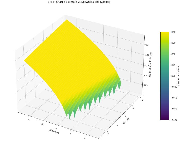
\begin{equation}\hat{\sigma}(\widehat{S})=\sqrt{\frac{1}{n-1}\left(1+\frac{1}{2} \widehat{S}^{2}\right)}\end{equation}

Normality assumption on returns could in fact be dropped, and still the estimated Sharpe ratio would follow a Normal distribution. Where Gamma3 and Gamma4 denote the skewness and kurtosis of the distribution of returns, the STD of the estimate is

\begin{equation}\hat{\sigma}(\widehat{S})=\sqrt{\frac{1}{n-1}\left(1+\frac{1}{2} \widehat{S}^{2}-\gamma_{3} \widehat{S}+\frac{\gamma_{4}-3}{4} \widehat{S}^{2}\right)}\end{equation}

As a solution for the problems discussed previously, we get the Probabilistic Sharpe Ratio (PSR) which is just the probability that the Sharpe is above some benchmark i.e.

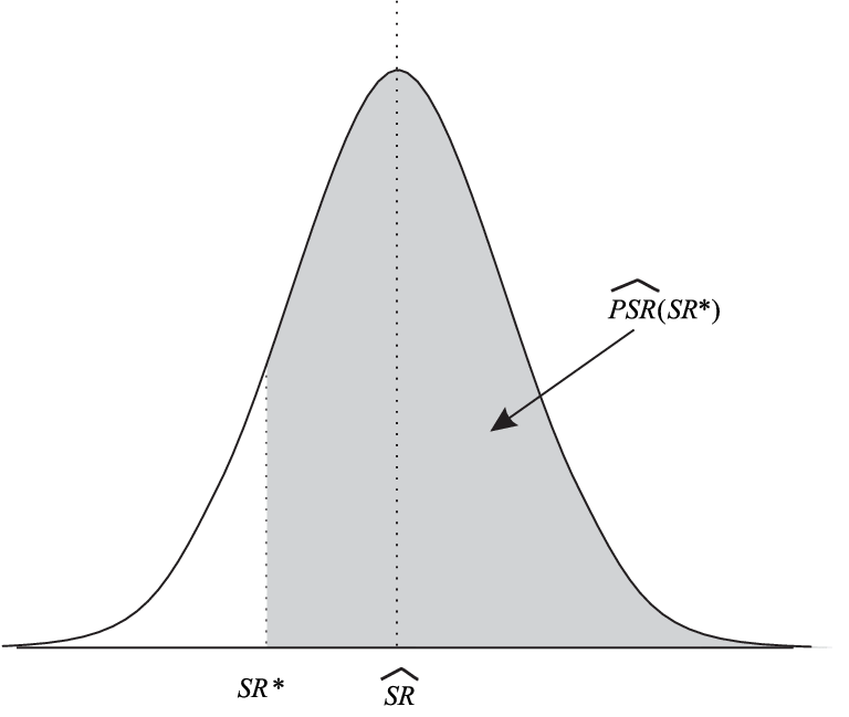
\begin{equation}P S R\left(S ^{*}\right)=\mathbb{P}[S^* \leq \widehat{S }]\end{equation}

Where Φ is the CDF of the Standard Normal Distribution, S* is the benchmark Sharpe, n is the number of observations, and skewness (gamma3) and kurtosis (gamma4) are the third and fourth standardized moments, we can show that

\widehat{P S R}\left(S^{*}\right)=\Phi\left[\frac{\left(\widehat{S}-S^{*}\right)}{\hat{\sigma}(\widehat{S})}\right] =\Phi\left[\frac{\left(\widehat{S}-S^{*}\right) \sqrt{n-1}}{\sqrt{1+\frac{1}{2} \widehat{S}^{2}-\gamma_{3} \widehat{S}+\frac{\gamma_{4}-3}{4} \widehat{S}^{2}}}\right]

The Minimum Track Record Length

We note that the PSR formula allows us to establish the track record length needed for rejecting the hypothesis that a measured Sharpe ratio is below a certain threshold with a given confidence level and model the trade-off between track record length and undesirable statistical features of negative skewness and positive excess kurtosis.

The graph below shows the number of observations required for the PSR to exceed 0.95 with a benchmark of 0.5 when the true Sharpe of the underlying generative process is 1 in the case where returns are normally distributed, versus when there is -3.5 skew and 10 kurtosis. The code is given in the appendix.

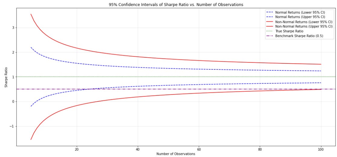
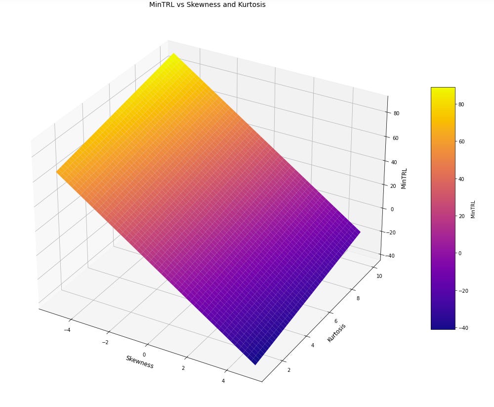
Negative skewness, which indicates a higher likelihood of large negative returns, and excess kurtosis, which reflects heavy tails or extreme outliers, both increase the uncertainty around the Sharpe Ratio estimate. This uncertainty decreases the PSR, and simultaneously increase the minimum amount of data required to confidently assess that the observed Sharpe Ratio is above the benchmark, i.e. the Minimum Track Record length (MinTRL). In particular, where

\text{MinTRL} = n^* = \text{Min} (n \mid \hat{PSR}(S^*) > 1 - \alpha)

the MinTRL is given by

\text{MinTRL} = n^* = 1 + \left[ 1 - \hat{\gamma}_3 \hat{S} + \frac{\hat{\gamma}_4 - 1}{4} \hat{S}^2 \right] \left( \frac{\Phi(\alpha)}{\hat{S} - S^*} \right)^2

The Sharpe Efficient Frontier

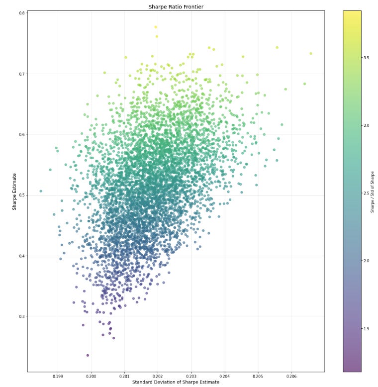
PSR evaluates the performance of an individual investment in terms of an uncertainty-adjusted SR. It seems natural to extend this argument to a portfolio optimization or capital allocation context. Unlike the traditional Markowitz mean-variance efficient frontier, which maximizes portfolio returns for a given level of risk on capital, the Sharpe Efficient Frontier identifies the set of portfolios that deliver the maximum expected Sharpe Ratio, subject to the uncertainty surrounding their point estimates.

Below are 5000 random portfolios formed from selecting among stocks in the NASDAQ 100 over the last 20 years of data.

Recap

The Sharpe Ratio, a measure of risk-adjusted returns, is prone to inflation from sampling variability and higher moments in returns. The PSR addresses this by quantifying the probability that a Sharpe Ratio exceeds a benchmark, accounting for higher moments like skewness and kurtosis. Negative skewness and excess kurtosis increase uncertainty, lowering PSR and extending MinTRL, highlighting the trade-off between track record length and undesirable return distribution features.

The Sharpe Efficient Frontier (SEF) extends PSR to portfolio optimization by identifying portfolios that maximize expected Sharpe Ratios while incorporating uncertainty in their estimates. SEF offers a robust alternative to mean-variance optimization, adjusting for non-Normal returns and finite sample sizes. Together, these tools enable more informed, uncertainty-aware portfolio decisions under real-world complexities.

Appendix: Code for PSR & MinTRL

import numpy as np
import matplotlib.pyplot as plt
from scipy.stats import norm

# Parameters for the true Sharpe Ratio
SR_hat = 1
benchmark_sharpe = 0.5

# Function definitions
def standard_deviation_sharpe_ratio(sharpe_ratio, num_obs, skewness=0, kurtosis=3):
    """Estimates standard deviation of Sharpe Ratio."""
    return np.sqrt(
        (1 - skewness * sharpe_ratio +
         (kurtosis - 1) / 4 * sharpe_ratio ** 2) / (num_obs - 1)
    )

def two_sided_confidence_intervals(sharpe_ratio, standard_deviation, confidence_level=0.95):
    """Calculates two-sided confidence intervals for the Sharpe Ratio."""
    alpha = 1 - confidence_level
    Z_alpha_over_2 = norm.ppf(1 - alpha / 2)
    lower_bound = sharpe_ratio - Z_alpha_over_2 * standard_deviation
    upper_bound = sharpe_ratio + Z_alpha_over_2 * standard_deviation
    return lower_bound, upper_bound

# Range of number of observations
num_obs_range = np.arange(5, 101, 1)

# Initialize lists for confidence intervals
ci_norm_lower = []
ci_norm_upper = []
ci_non_norm_lower = []
ci_non_norm_upper = []

# Compute confidence intervals for each number of observations
for N in num_obs_range:
    sigma_norm = standard_deviation_sharpe_ratio(SR_hat, N, skewness=0, kurtosis=3)
    sigma_non_norm = standard_deviation_sharpe_ratio(SR_hat, N, skewness=-3.5, kurtosis=10)
    
    lower_norm, upper_norm = two_sided_confidence_intervals(SR_hat, sigma_norm)
    lower_non_norm, upper_non_norm = two_sided_confidence_intervals(SR_hat, sigma_non_norm)
    
    ci_norm_lower.append(lower_norm)
    ci_norm_upper.append(upper_norm)
    ci_non_norm_lower.append(lower_non_norm)
    ci_non_norm_upper.append(upper_non_norm)

# Plotting
plt.figure(figsize=(18, 8))

# Plot confidence intervals for normal returns
plt.plot(num_obs_range, ci_norm_lower, label="Normal Returns (Lower 95% CI)", color="blue", linestyle="--")
plt.plot(num_obs_range, ci_norm_upper, label="Normal Returns (Upper 95% CI)", color="blue", linestyle="--")

# Plot confidence intervals for non-normal returns
plt.plot(num_obs_range, ci_non_norm_lower, label="Non-Normal Returns (Lower 95% CI)", color="red")
plt.plot(num_obs_range, ci_non_norm_upper, label="Non-Normal Returns (Upper 95% CI)", color="red")

# True Sharpe Ratio
plt.axhline(SR_hat, color="green", linestyle=":", label="True Sharpe Ratio")

# Benchmark Sharpe Ratio
plt.axhline(benchmark_sharpe, color="purple", linestyle="-.", label="Benchmark Sharpe Ratio (0.5)")

# Labels and legend
plt.title("95% Confidence Intervals of Sharpe Ratio vs. Number of Observations")
plt.xlabel("Number of Observations")
plt.ylabel("Sharpe Ratio")
plt.legend()
plt.grid(alpha=0.3)

# Show plot
plt.show()

Disclaimer

The information provided on TheLogbook (the "Substack") is strictly for informational and educational purposes only and should not be considered as investment or financial advice. The author is not a licensed financial advisor or tax professional and is not offering any professional services through this Substack. Investing in financial markets involves substantial risk, including possible loss of principal. Past performance is not indicative of future results. The author makes no representations or warranties about the completeness, accuracy, reliability, suitability, or availability of the information provided.

This Substack may contain links to external websites not affiliated with the author, and the accuracy of information on these sites is not guaranteed. Nothing contained in this Substack constitutes a solicitation, recommendation, endorsement, or offer to buy or sell any securities or other financial instruments. Always seek the advice of a qualified financial advisor before making any investment decisions.