


There is one coherent regime which makes sense for rates and stocks to rise together rapidly: markets pricing a non-trivial probability of AGI. Higher expected future consumption pushes households to borrow against it, lifting real rates; higher expected future earnings lift equity prices, with the joint move’s magnitude pinned to a single elasticity. This post explains the claim, from intuition through formalism, EMH priors, 35 years of cross-country panel evidence, and a calibrated read of where current rates imply the market’s AGI probability sits. The primary reference is Transformative AI, existential risk, and real interest rates by Halperin, Chow, and Mazlish.
The Relationship Between Rates & Growth
The link between “expected to be rich in the future” and “high interest rates today” is the one most counterintuitive piece of the argument for non-economists, so let us build it up before formalizing.
Suppose you learn today, with perfect certainty, that you will inherit $100 million in five years. What do you do?
Most people asked the question directly say something like: take out a loan now, buy a house, take a sabbatical, start a business. The thing all those answers have in common is that they involve borrowing against the future windfall. You do not need to save for retirement anymore, because retirement is taken care of. You do not need to maintain a precautionary buffer, because the buffer is on the way. The marginal dollar five years from now is worth much less to you than the marginal dollar today, because in five years you will have so many dollars that one more makes very little difference to your life, while today every dollar still has a noticeable effect.
You would also be willing to pay quite a lot of interest on that loan. If a bank offered you a five-year loan at 15% annualized, you would probably take it, because 15% on a small loan today is paid back from a much larger pile in five years. The high rate does not deter you. The rate that does deter you is the rate that exceeds the implicit “exchange rate” between your current dollar-poor self and your future dollar-rich self, which is a high rate indeed.
Now imagine the same thing, but not just for you. Imagine everyone learns today that AGI will arrive in five years and they will all be much richer than they currently are. What does the loan market look like?
Demand for loans is high (everyone wants to borrow against the future). Supply of loans is low (why save when you are about to be rich anyway). With high demand chasing low supply, the price of loans, which is the interest rate, rises. It rises a lot. The market clears at whatever rate equates the smaller pool of people willing to delay consumption against the larger pool of people who want to consume now and pay back later. This is the whole mechanism. Expected future wealth raises interest rates because it shifts both sides of the loanable-funds market in the same direction.
Households have a strong preference to smooth consumption across time. A consumption path of $100 today, $100 next year, $100 the year after that feels much better than a path of $50 today, $200 next year, $50 the year after that, even though both have the same total dollar value. The reason is diminishing marginal utility: the second hundred dollars in a single year is less valuable than the first hundred.
Take this preference seriously and combine it with an expectation that future consumption will be much higher. The household sees a future of $1000K a year (post-AGI prosperity) and a present of $100K a year. The smoothing preference says this is a bad allocation. The household would rather have, say, $400K a year for both present and future. To get from $100K today to $400K today, it has to consume more than it earns today, which means borrowing.
It is willing to pay quite a bit to do so, because the $400K it wants to spend today is worth much more in utility terms than the $400K of future income it gives up. The interest rate it is willing to pay is bounded by how much it values the smoothing. Aggregate this across all households, and the same conclusion follows. The economy-wide interest rate rises because everybody wants to do the same kind of borrowing.
The Ramsey Rule Formalized
With the intuition in hand the formal version is a single equation away. Start with the canonical consumption-Euler equation. A household with time-separable utility u(C), subjective discount factor β ∈ (0, 1], and survival probability δ ∈ (0, 1] solves an intertemporal allocation problem whose first-order condition is
The survival probability δ represents a chance that the household might not be around tomorrow to enjoy future consumption, so it discounts the future more. Under isoelastic utility u(C) = C^(1 − 1/σ) / (1 − 1/σ) with elasticity of intertemporal substitution σ, perfect foresight, and constant consumption growth g, this collapses to the Ramsey rule
where ρ bundles time preference and survival into a discount parameter (ρ ≈ −ln(βδ)). Each term has an interpretation:
ρ is the rate at which households discount the future for impatience and mortality reasons alone, even at constant consumption.
g is the expected growth rate of consumption.
1/σ measures how much the household dislikes intertemporal consumption inequality. Higher 1/σ (lower σ) means a stronger desire to smooth, which translates into a stronger willingness to pay for borrowing when the future is expected to be richer.
Add uncertainty in growth. With log-normally distributed consumption growth (mean g, variance Var(g)) and isoelastic utility, the rule becomes
The new term is precautionary savings: uncertainty about future consumption raises desired saving, which pushes rates down. In the limit of certain growth, this term vanishes. In the limit of very uncertain growth, this term can be large enough to offset most or all of the growth effect.
Empirical Evidence
Real rates predict realized GDP growth: take inflation-linked bond yields (TIPS in the US since 1999, indexed gilts in the UK since 1985, Australian and Canadian linkers since the mid-1990s), and plot them against subsequent realized GDP growth over 10-, 15-, and 20-year horizons. If the Ramsey rule is doing real work, higher real yields should predict higher subsequent growth, because the real yield is the market’s pricing of expected growth on average.
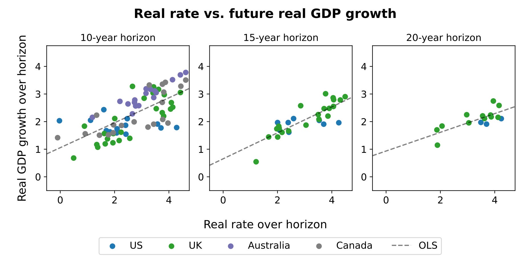
The relationship is noisy because long-horizon predictions involve a lot of unrealized future variance, but the sign is right and the slope is meaningful. This is the sanity check on the equivalent claim in the other direction: when markets expect higher growth, they bid up real yields. The same dataset that lets the paper estimate the EIS at 0.74 also says the rate-growth link is empirically real and not an artefact of theory.
The deeper test is a panel regression with Consensus Economics survey-based growth forecasts on the right-hand side and inflation-linked sovereign yields on the left-hand side, across 59 countries from approximately 1990 to today. The dependent variable is the 5-year-forward 5-year real rate (the rate from year 5 to year 10 implied by current bond prices). The key right-hand-side variable is the Consensus Economics 5-year-forward 5-year GDP growth forecast. Controls include the standard deviation of the forecast, the 0-to-5-year growth forecast, and 10-year sovereign CDS spread. Standard errors are Driscoll-Kraay to handle cross-country correlation.
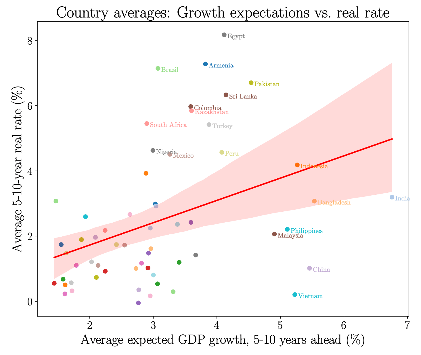
The labeled country scatter is striking. Across-country variation alone produces a strong positive slope. The clear anomaly is China and Vietnam, which combine high growth expectations with low real rates. The paper interprets this as evidence of capital controls preventing the rate-growth link from binding in countries with restricted external capital flows. Strip those out and the relationship is even cleaner.
The empirical conclusion is that the Ramsey-rule slope holds in the data. Real rates do in fact move with expected growth, by roughly the amount the theory predicts. This validates using observed rate movements to back out implied growth-expectation changes, and therefore validates using observed rate movements to back out implied probability shifts on regime-change scenarios like AGI.
Aligned & Unaligned AI
The Euler equation has two parameters that move with AI scenarios. Aligned AI moves g (expected consumption growth) up substantially. Unaligned AI moves δ (survival probability) down substantially. Both push the equilibrium real rate up.
The growth channel is what we previously covered. The survival channel is worth developing on its own. Take the Euler equation and solve for the implicit relationship between r and the discount parameters
If δ falls (survival probability drops), the term −ln(βδ) rises. A 1% per year drop in survival probability translates roughly to a 1 percentage point rise in real rates. The intuition: if there is a non-trivial chance you will not be alive next year, you discount future consumption more heavily, which is the same thing as demanding a higher return to delay current consumption.
This is empirically grounded. We see it in several historical episodes:
AIDS antiretroviral rollout in Malawi (Baranov-Kohler 2018): when aid arrived and life expectancy rose by roughly 13 years, household savings rates rose measurably and investment in human capital (schooling) increased. The survival-probability shock was visible in aggregate decisions.
Sri Lankan mortality drop, 1946-53 (Jayachandran-Lleras-Muney 2009): every additional year of life expectancy translated to 0.11 additional years of schooling. The mechanism: parents invest more in children’s human capital when those children are likelier to live long enough to use it.
Huntington’s disease testing (Oster-Shoulson-Dorsey 2013): people who learn they are positive for Huntington’s complete college at rates roughly 30 percentage points lower than those who learn they are negative. Survival probability shocks change life-cycle decisions on time horizons that match the savings response.
These episodes confirm the survival-probability channel runs in the right direction at the household level. The unaligned-AI scenario in Halperin et al. has people putting nontrivial probability on existential risk over the next several decades. Even modest probability estimates, say 1% per year of extinction-level catastrophe, translate to roughly a 1 percentage point rise in real rates through the survival channel.
The important point is that both AI scenarios push rates up. Aligned AI raises g, which raises r via the growth channel. Unaligned AI lowers δ, which raises r via the survival channel.
The Recent Path of Rates
US 10-year TIPS real yields bottomed at roughly −1.0% in late 2021. They have risen steadily since, and long-dated yields across the developed world have continued to push higher: 30-year sovereigns in the US, UK, France, and Japan are now trading at nominal yields in the 5–6% range across the long end. That is roughly a 450 to 600 basis point move on the long end from the 2021 trough.
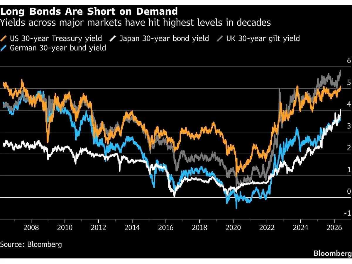
The popular explanation is fiscal dominance: unsustainable deficits, debt-to-GDP grinding higher, and term premium re-emerging as the marginal buyer of long-dated paper questions whether the issuer can credibly stabilize the path of debt. There is a real case for this. Deficits are large and structural, and it is not clear that necessary cuts to popular entitlement programs are politically viable.
But it is not the only story consistent with what we are observing. The Ramsey rule under uncertainty is linear in probability
solving for the implied probability p given an observed r gives
The point of the framework is that anything which shifts expected future consumption growth, fiscal-driven supply pressure, demographic re-pricing, or rising probability of transformative AI, feeds into the same real-rate observable. Fiscal dominance and AGI repricing are observationally adjacent on the rate channel. The first does not falsify the second; they would coexist in the same long-yield path.
Plug today’s roughly 3% real long-end rate into the calibration with ρ = 1%, g_TAI = 30%: the implied probability runs ≈5% at σ = 0.74, ≈7% under log utility (σ = 1), and ≈10% under an asset-pricing-prior σ = 1.5.
The Forecasting Research Institute’s elicitation of 69 economists puts the median probability of a rapid-AI scenario by 2030 at 10%, with an interquartile range of 6.7 to 20%. The implied rate-based probabilities sit roughly inside this range. The market is not “strongly rejecting” near-term AGI under any defensible reading of the long end; it is pricing a single-digit-to-low-double-digit probability, which is approximately what professional forecasters say.
Plug today’s roughly 5% real long-end rate with ρ = 1%, g_AGI = 30%: the implied probability runs ≈10% at σ = 0.74, ≈13% under log utility (σ = 1), and ≈20% under an asset-pricing-prior σ = 1.5.
The Forecasting Research Institute’s elicitation of 69 economists puts the median probability of a rapid-AI scenario by 2030 at 10%, with an interquartile range of 6.7 to 20%. The rate-implied probabilities sit on the FRI median and span its full interquartile range. The market is not just consistent with single-digit AGI pricing; it is consistent with the central tendency of professional forecasters, and at the high-EIS end with the upper quartile.
A nuance about which “AGI growth rate” to use in the calibration. The 30% benchmark is at the high end; FRI economists who put 10% probability on a “rapid AI scenario” by 2030 expect, conditional on that scenario, GDP growth of only 3.3 to 3.5%, an order of magnitude lower.
If the market is pricing a milder rapid-AI scenario (say, 5% growth instead of 30%), the implied probability from the observed rate rise climbs to 60% or higher. The framework is sensitive to the assumed conditional growth rate; pick a lower g_AGI and the implied probability is much higher for the same observed rate.
The Joint Move with Stocks
Take the Gordon equation in the simplest form
A pure rates-up shock with g_D unchanged drops P unambiguously. A pure growth-up shock with r unchanged raises P unambiguously. A simultaneous shock where both r and g_D rise leaves the sign of P’s change ambiguous. The relative sizes matter.
Aligned AGI raises both the numerator (profits) and the denominator (the discount rate that prices those profits), and the net sign depends on the elasticity of intertemporal substitution. The condition turns out to be:
σ > 1: the growth effect dominates and equities rise on a AGI shock.
σ < 1: the discount effect dominates and equities fall on a AGI shock.
σ = 1: the two effects approximately cancel and equities are roughly unchanged.
A quick reminder on what σ, the EIS, is actually saying. EIS measures how much a household will shift its consumption-growth path in response to a change in rates.
Low EIS (σ around 0.5) means households are sticky about smoothing: they want roughly the same standard of living year to year and need large rate moves to budge their savings decisions. High EIS (σ around 2) means households are flexible: a higher rate is a great deal, so they happily cut spending now to consume more later. Log utility (σ = 1) is the textbook middle case.
Macro consumption-Euler estimates of the EIS in the broader literature cluster at σ between 0.2 and 1. Under this prior, AGI being priced in implies equities fall, not rise. The current pattern of both rates rising and equities rising is in that case inconsistent with the AGI hypothesis.
But the asset-pricing literature reaches the opposite conclusion. Long-run-risks models, recursive utility calibrations consistent with the equity premium, and the macro-finance term-structure literature all calibrate σ at values above 1, typically 1.5 to 2. Under this prior, AGI raises equities.
There is no settled answer to which σ is right. The empirical consumption-Euler literature has historically said low, the asset-pricing literature has historically said high, and the gap between them has not closed in 40 years.
If you believe the macro-Euler σ, the joint move is evidence against AGI being priced. If you believe the asset-pricing σ, it is evidence for. Given the asset-pricing prior, current markets are consistent with low-double-digit AGI probability being priced. Given the macro-Euler prior, they are not.
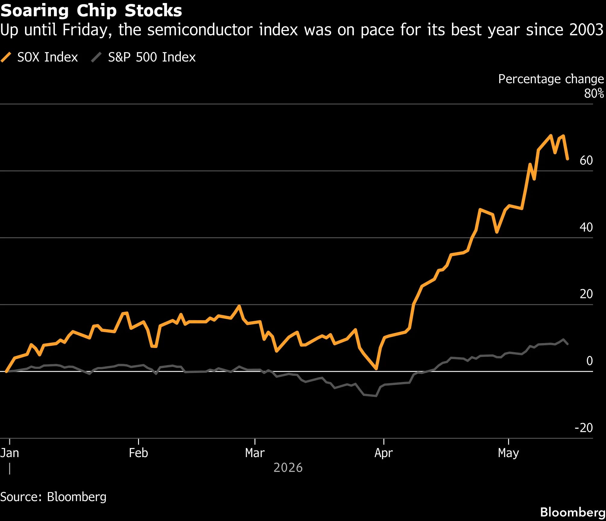
Stocks are a Bad Signal for AGI Risk
Setting aside the EIS-sign-ambiguity problem, there are three other independent reasons stocks are a worse direct signal of AGI than rates are.
Alignment risk zeroes everything. In the unaligned scenario, equities, bonds, and currency all go to zero. So a meaningful portion of the probability mass on transformative AI sends the equity price to zero regardless of which companies were positioned to benefit. The equity level is already adjusted for that wipeout probability, and disentangling the alignment piece from the underlying-business piece is not identified. Rates do not have this problem: the survival channel pushes them up under unalignment, the growth channel pushes them up under alignment, and the observed rate carries a clean signal of total AI probability.
Profit capture is uncertain even conditional on aligned AI. If 30%/year GDP growth materializes, who captures the surplus? There are several reasons public-equity holders may not: explicit profit caps (OpenAI’s original 100x cap), Windfall Clause-style precommitments to redistribute, government expropriation or nationalization, and simple competitive dispersion that splits the surplus across thousands of firms so that no single one captures much. Each of these is a path on which “aligned AGI arrives” coexists with “current public-equity valuations were not justified by the AGI thesis.”
The most AGI-relevant firms are private. The auto industry was transformative for the 20th-century economy, but most equity investors who tried to capture the auto boom in the 1900s and 1910s lost money to bankruptcies and dilution; the surviving giants mostly were not public during the formative period. Today’s analog is direct: the leading labs (OpenAI, Anthropic, xAI) are predominantly private. Public-equity investors have to bet on adjacent firms, NVDA, MSFT, semi equipment, rather than the labs themselves, and if value capture happens at the lab level it is invisible to public-equity prices.
Conclusions
None of the above arguments show that the AGI hypothesis is indeed what is driving rates and stocks up together. There are many candidate stories: fiscal dominance, structural shifts in the savings-investment balance, demographic re-pricing, an inflation regime change, term-premium normalization. Most of them have real evidence behind them, and on a simple weighting of priors the AGI explanation is not the largest single contributor to what we are seeing.
Nonetheless, the AGI hypothesis is one explanation that is consistent with the full joint pattern rather than just the rates side. A world where the market is gradually shifting weight onto a non-trivial near-term AGI probability looks like exactly what we have: earnings expanding rapidly as firms capture AI-driven productivity, equity prices climbing the wall of worry over higher rates and stickier inflation, and earnings pulling ahead of price fast enough to absorb the discount-rate move.
Climbing rates do not have to kill the equity story if the growth story is moving faster. So the calibrated read is not “this is a bubble” and not “AGI is priced in.” It is that AGI risk is one out of several plausible drivers, that under a defensible-but-not-settled choice of prior it could be a meaningful share of the joint move, and that on the rate-implied calibration the market is already pricing a probability that sits at the central tendency of professional forecasters.
Disclaimer
The information provided on TheLogbook (the “Substack”) is strictly for informational and educational purposes only and should not be considered as investment or financial advice. The author is not a licensed financial advisor or tax professional and is not offering any professional services through this Substack. Investing in financial markets involves substantial risk, including possible loss of principal. Past performance is not indicative of future results. The author makes no representations or warranties about the completeness, accuracy, reliability, suitability, or availability of the information provided.
This Substack may contain links to external websites not affiliated with the author, and the accuracy of information on these sites is not guaranteed. Nothing contained in this Substack constitutes a solicitation, recommendation, endorsement, or offer to buy or sell any securities or other financial instruments. Always seek the advice of a qualified financial advisor before making any investment decisions.