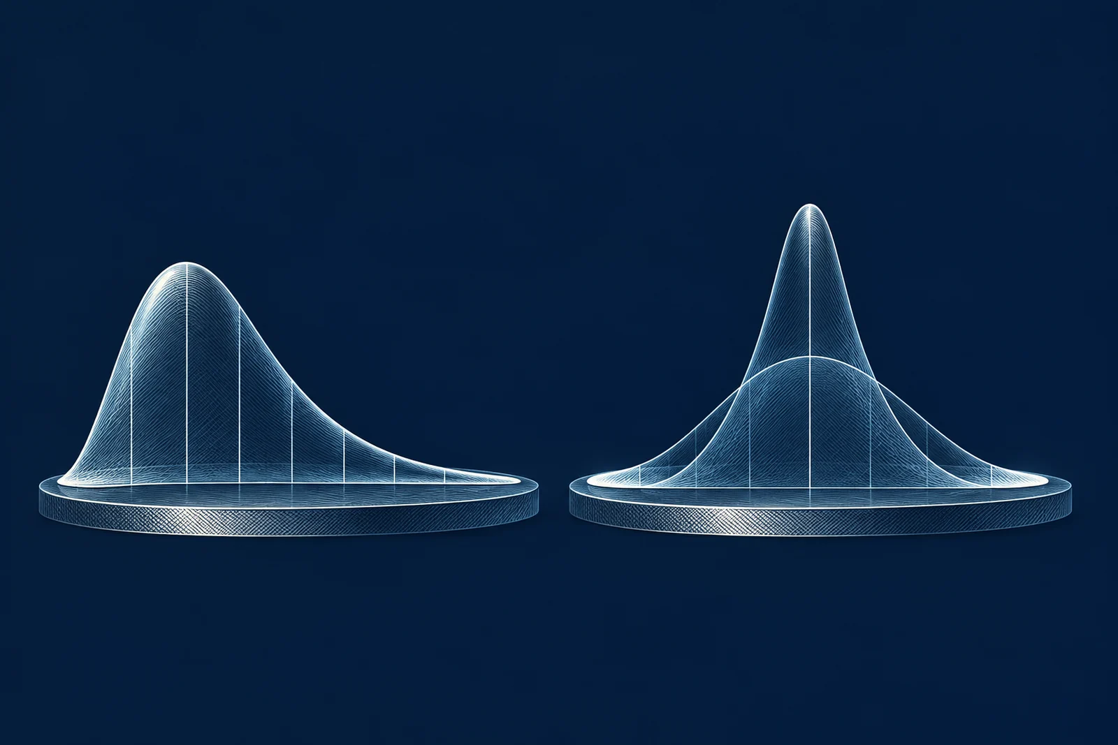
Skew and Kurtosis from Two Perspectives

From The Logbook. The original article is reproduced in full, with minor grammar corrections; references to market conditions reflect the context in which it was written.

Skew and kurtosis in implied volatility distributions provide key insights into both the dynamics of underlying assets and the distribution of its final price. Skew, which measures the asymmetry of the distribution, can be interpreted as an indicator of spot-volatility correlation. Kurtosis, which measures the "tailedness" of the distribution, is somewhat related to the volatility of volatility. In this short post, we provide some intuition as to how models of the underlying dynamic (spot-vol correlation (i.e. local volatility) and vol of vol (i.e. stochastic volatility)) are related to models of the underlying’s price at expiration (asymmetry, fat tails).

Skew and Spot-Vol Correlation / Local Volatility

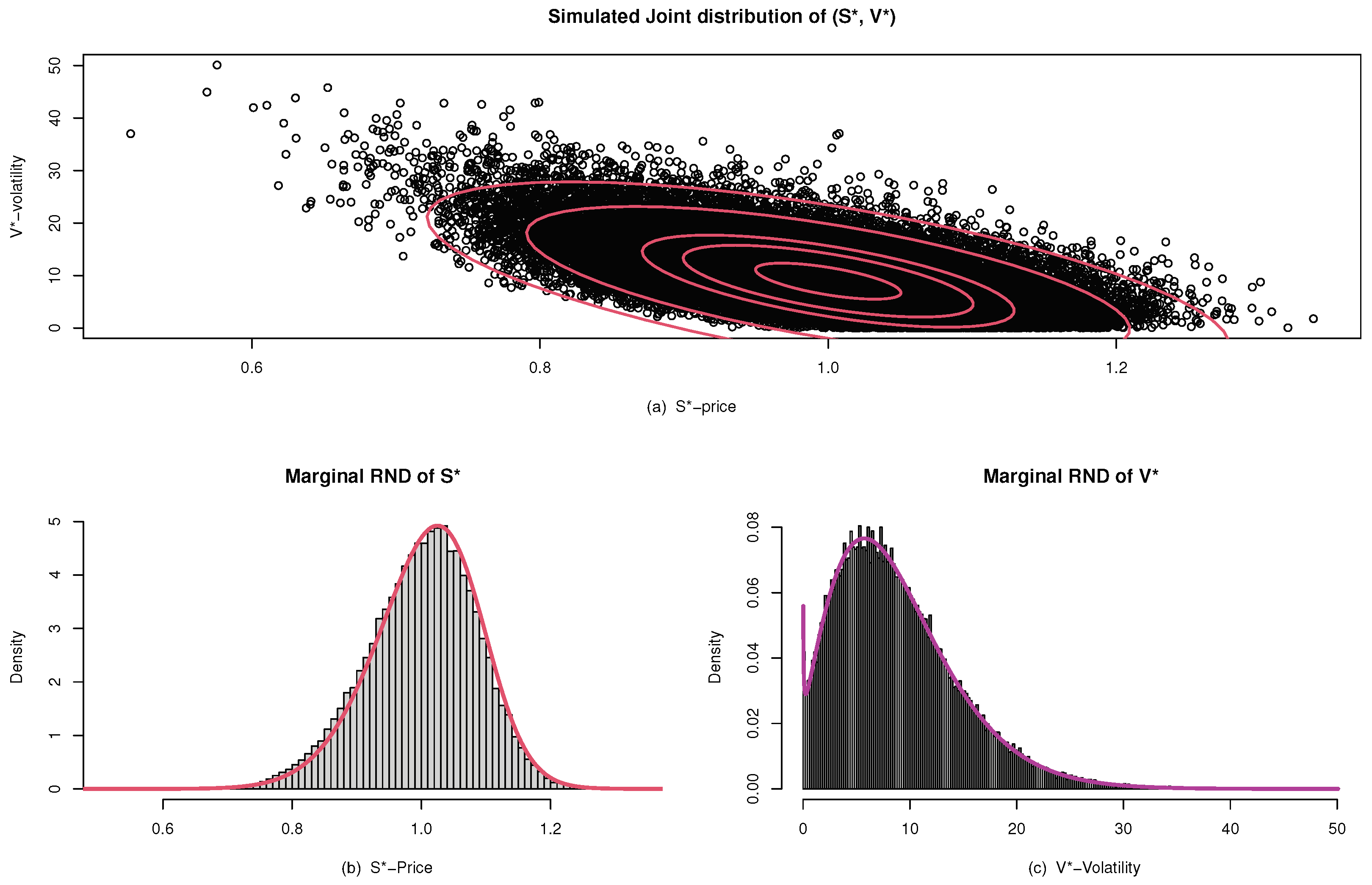
Suppose we were pricing a far downside put and far upside call. Assume a strongly negative correlation between spot price and instantaneous volatility. We first consider the effects on pricing (think Monte Carlo in terms of paths is helpful here). For the put, it is the strongly bearish paths that will matter i.e. only the paths that finish below the strike (why? because an option can be replicated not only by continuous delta hedging but also by delta hedging only at the strike) where the spot is expected to strongly decrease; due to negative spot-vol correlation, along these bearish paths vol is expected to increase, thus making strike volatility high. The same argument applies to the call side, and strike vol should be low there consequently. This shows that spot-vol correlation should induce skew in the risk-neutral distribution.

The alternative way to think about this is that if the spot price moves more significantly when it decreases than when it increases, there needs to be a compensatory mechanism to maintain a balanced mean or fair current spot price. This results in a pronounced down tail in the distribution, where the average extent of downward movements must exceed that of upward movements to offset the lesser frequency or magnitude of spikes when prices rise. As such, the local volatility induced by spot-vol correlation must again induce skew in the implied distribution.

Interpretations of Correlation

This is a side note and completely unrelated to the rest of the post, but I’ve noticed that many professionals don’t actually know this very intuitive definition of correlation and instead just vaguely interpret it as a measure of linear dependence.

Specifically, correlation measures the strength and direction of a linear relationship between two variables. It essentially tells us how well one variable predicts the other when they are both standardized, meaning when we look at changes in terms of standard deviations from their means. When one variable moves one standard deviation away from its mean, correlation is our best guess of how many standard deviations the other variable moves from its mean.

When we calculate correlation, we normalize covariance by the product of the standard deviations of the two variables. This normalization ensures that the correlation coefficient remains between -1 and 1. Conceptually, if a correlation were to exceed 1, it would imply that the combined movements of the variables are more extreme than could be accounted for by their individual spreads (standard deviations). This is mathematically impossible because it would mean the covariance between the variables is greater than the product of their standard deviations, suggesting a relationship stronger than perfect synchrony.

When the correlation is exactly 1, every point in the sample space lies perfectly on a straight line with a positive slope. This indicates that for every unit change in one variable, there is a proportional and consistent unit change in the other variable, matched exactly by the ratio of their standard deviations. This perfect alignment shows that all variability in one variable can be linearly explained by the other with no residual variance—every point is exactly as spread out from the line as dictated by their standard deviations; hence r-squared would also be 1.

Interpretations of Kurtosis

Before discussing the relationship between kurtosis and vol of vol, it is perhaps useful to think about what kurtosis actually is. Specifically, per Wikipedia

[Kurtosis] reflects either the presence of existing outliers (sample kurtosis) or the tendency to produce outliers (kurtosis of a probability distribution). The underlying logic is straightforward: Kurtosis represents the average of standardized data raised to the fourth power. Standardized values less than 1—corresponding to data within one standard deviation of the mean (where the “peak” occurs)—contribute minimally to kurtosis. This is because raising a number less than 1 to the fourth power brings it closer to zero. The meaningful contributors to kurtosis are data values outside the peak region, i.e., the outliers. Therefore, kurtosis primarily measures outliers and provides no information about the central "peak".

Numerous misconceptions about kurtosis relate to notions of peakedness. One such misconception is that kurtosis measures both the “peakedness” of a distribution and the heaviness of its tail. Other incorrect interpretations include notions like “lack of shoulders” (where the “shoulder” refers vaguely to the area between the peak and the tail, or more specifically, the region about one standard deviation from the mean).

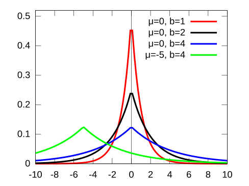
The above misconceptions capture intuition about kurtosis in peaked distributions such as the Laplace family of distributions, which have excess kurtosis

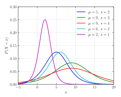
However, it fails when it comes to examples such as the logistic family of distributions, which have round peaks and also excess kurtosis

Returning to the definition of kurtosis, we can be more specific if we use notation. The kurtosis of a random variable X can be interpreted by the standardized

Z={\frac {X-\mu }{\sigma }}

we can show that

{\begin{aligned}\kappa &=\operatorname {E} \left[Z^{4}\right]\\&=\operatorname {var} \left[Z^{2}\right]+\operatorname {E} {\!\left[Z^{2}\right]}^{2}\\&=\operatorname {var} \left[Z^{2}\right]+\operatorname {var} [Z]^{2}=\operatorname {var} \left[Z^{2}\right]+1.\end{aligned}}

Which shows that the kurtosis is a measure of the dispersion of Z² around its expectation. In terms of the original variable X, the kurtosis is a measure of the dispersion of X around the two values μ ± σ.

Kurtosis and Vol of Vol / Stochastic Volatility

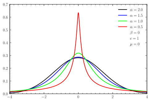
A tempting, but ultimately incorrect intuition is to consider the implied distribution of the spot price as a superposition three distributions representing low, medium, and high volatility states that are possible due to stochastic volatility; a sharp peak for low volatility, a broader distribution for normal conditions, and fat tails for high volatility periods. However, this interpretation has limitations since superposing normal distributions inherently results in another normal distribution (no excess kurtosis like the Levy distributions below).

Instead, let us ask an slightly different question: what type of underlying generative process makes it difficult for us to know what vol is? That is to say, when is the variance of sample variance high? In the case that Xi are independent observations from a normal distribution, Cochran's theorem shows that the unbiased sample variance S2 follows a scaled chi-squared distribution

(n-1){\frac {S^{2}}{\sigma ^{2}}}\sim \chi _{n-1}^{2}

\operatorname {E} \left(S^{2}\right)=\operatorname {E} \left({\frac {\sigma ^{2}}{n-1}}\chi _{n-1}^{2}\right)=\sigma ^{2}

{ {Var} \left[S^{2}\right]=\operatorname {Var} \left({\frac {\sigma ^{2}}{n-1}}\chi _{n-1}^{2}\right)={\frac {\sigma ^{4}}{{\left(n-1\right)}^{2}}}\operatorname {Var} \left(\chi _{n-1}^{2}\right)={\frac {2\sigma ^{4}}{n-1}}}

We can see that the var of var (and hence vol of vol) in the underlying distribution contributes to var of sample var, but for normal distributions there is no excess kurtosis and naturally the term does not emerge. However, if Xi are independent and not necessarily normal then we can rewrite the sample variance S2 as an average over all pairs of indices (Source: Introduction to the Theory of Statistics, Mood, Graybill, Boes, 3rd Edition, 1974, p. 229):

S^2={1\over{n\choose 2}}\sum_{\{i,j\}} {1\over2}(X_i-X_j)^2.

The variance of S2 is the expected value of

\left({1\over{n\choose 2}}\sum_{\{i,j\}} \left[{1\over2}(X_i-X_j)^2-\sigma^2\right]\right)^2.

When you expand the outer square, there are 3 types of cross product terms

\left[{1\over2}(X_i-X_j)^2-\sigma^2\right] \left[{1\over2}(X_k-X_\ell)^2-\sigma^2\right]

depending on the size of the intersection {i,j}∩{k,ℓ}. When this intersection is empty, the factors are independent and the expected cross product is zero. There are n(n−1)(n−2) terms where |{i,j}∩{k,ℓ}|=1 and each has an expected cross product of (μ4−σ4)/4. There are (n2) terms where |{i,j}∩{k,ℓ}|=2 and each has an expected cross product of (μ4+σ4)/2. Putting it all together shows that

\text{Var}(S^2)={\mu_4\over n}-{\sigma^4\,(n-3)\over n\,(n-1)}

Using the identity μ4=(κ+3)σ4, we can finally show that

\operatorname {E} \left[S^{2}\right]=\sigma ^{2},\quad \operatorname {Var} \left[S^{2}\right]={\frac {\sigma ^{4}}{n}}\left(\kappa -1+{\frac {2}{n-1}}\right)={\frac {1}{n}}\left(\mu _{4}-{\frac {n-3}{n-1}}\sigma ^{4}\right)

This shows a dynamic of high volatility of volatility (high var of sample var, in some sense) can be attributed to either actually high var of var (σ4), or kurtosis (κ) in the underlying distribution itself. Just as the sampled mean (spot price) will move more if vol is actually higher, so too will the sampled variance (implied vol) move more either on actual uncertainty in implied vol or kurtosis in the underlying distribution. Put another way, kurtosis makes it difficult for us to know what the actual vol is, and its effects on dynamics can be indistinguishable from vol of vol under this framework.

When actual volatility of volatility is high, it indicates that the market's volatility is not only changing but doing so in an unpredictable manner (must be martingale else we can arbitrage). Kurtosis measures the tail heaviness of a distribution, pointing to a higher probability of realizing extreme values. High kurtosis complicates the interpretation of volatility because these extreme values skew the perceived stability or volatility of the market. Essentially, kurtosis adds an element of uncertainty to the estimation of volatility; extreme outcomes, which are more frequent in high-kurtosis environments, cause sampled variance (implied volatility) to swing more dramatically, mimicking the effects of genuine volatility fluctuations. In a practical sense, the effects of high kurtosis can sometimes be indistinguishable from those of actual volatility of volatility, and thus affecting the pricing of derivatives in the same way.

No Jumps Required

We distinguish between the impacts of kurtosis and discrete jumps. Kurtosis refers to the tail heaviness of a continuous distribution of returns, indicating a greater likelihood of extreme values within a purely continuous process. This contrasts with jumps, which are sudden, discrete shifts in asset values not predicted by standard diffusion models. I.e. jumps introduce unpredictability that requires different modeling approaches, such as incorporating jump-diffusion elements to capture sudden market moves accurately.

Stochastic Volatility Explains More than Kurtosis

Under an autocorrelated, mean-reverting, stochastic volatility framework, such as Heston, the term structure of volatility can be explained (this is not the case for merely incorporating kurtosis into the returns distribution). On a most basic level Heston explicitly incorporates mean reversion and volatility clustering into its structure, allowing for both levels the variance of volatility to be stochastic.

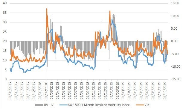
A natural consequence is that short-term volatilities tend to be lower under typical market conditions, reflecting market consensus that immediate volatility will remain close to its current, often subdued, level unless influenced by preceding factors. However, as the horizon extends, the term structure typically slopes upward, pricing in higher long-term volatilities to account for the increased probability of encountering volatility spikes at some point in the future. This long-term premium is a direct consequence of the model's allowance for volatility spikes driven by its mean-reverting and autocorrelated volatility processes.

When actual volatility spikes occur, the term structure inverts, with short-term volatilities jumping significantly above long-term expectations. This inversion reflects the autocorrelated nature of volatility under Heston: if current volatility is high, short-term future volatility is also likely to be high. However, long-term volatilities might not adjust as dramatically, given the mean-reverting property embedded in the model, which suggests that volatility will eventually revert to more typical levels.

We can observe this in the relationship between the S&P 500 past 30 day realized volatility and the VIX (the implied 30 day forward volatility)

Conclusions

In financial modeling, skew and kurtosis within implied volatility distributions provide deep insights into asset dynamics and price distributions at expiration. Skew, reflecting the asymmetry of the distribution, often results from a negative correlation between spot prices and volatility, suggesting that volatility increases when prices drop significantly. Kurtosis, indicating the heaviness of distribution tails, complicates the estimation of volatility by amplifying the effects of outliers, thus making it difficult to discern true volatility levels. However, a description of the final state of the risk-neutral distribution is ultimately not as powerful as a description of the underlying generative dynamic for the spot when it comes to pricing and trading options. For example, we see how stochastic volatility can explain the term structure of volatility while kurtosis itself cannot.