The Cost of Capital | Freeport Markets

From The Logbook. The original article is reproduced in full, with minor grammar corrections; references to market conditions reflect the context in which it was written.

The cost of capital is a fundamental concept in finance, yet it's often reduced to a mere plug-and-chug exercise in many classrooms. This oversimplification obscures the rich economic intuition associated with cost of capital calculations. At its core, the cost of capital represents the minimum return a company must earn on its investments to satisfy its providers of capital - both equity holders and creditors. It's not just a number to be calculated, but a reflection of risk, opportunity cost, and the balance between different sources of funding.

By delving deeper into the logic underpinning cost of capital calculations, we can gain valuable insights into how companies are assumed to make financial decisions, and how investors are assumed to evaluate opportunities. The main reference for this post is the paper Cost of Capital published by Morgan Stanley’s Counterpoint Global.

The Big Picture

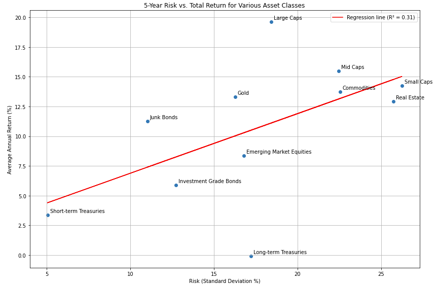
The cost of capital is the opportunity cost for investors in the setting of a diversified portfolio. The cost of capital is based on the principle of substitution: an investor will not invest in an asset if a comparable asset exists that has higher returns for the same level of risk or less risk for the same level of returns. This means that an investor will buy the asset with the highest return for a given level of risk, or the lowest risk for a given level of return. This assumes that risk is associated with reward; per CAPM, the two are linearly dependent under efficient markets (though not in reality).

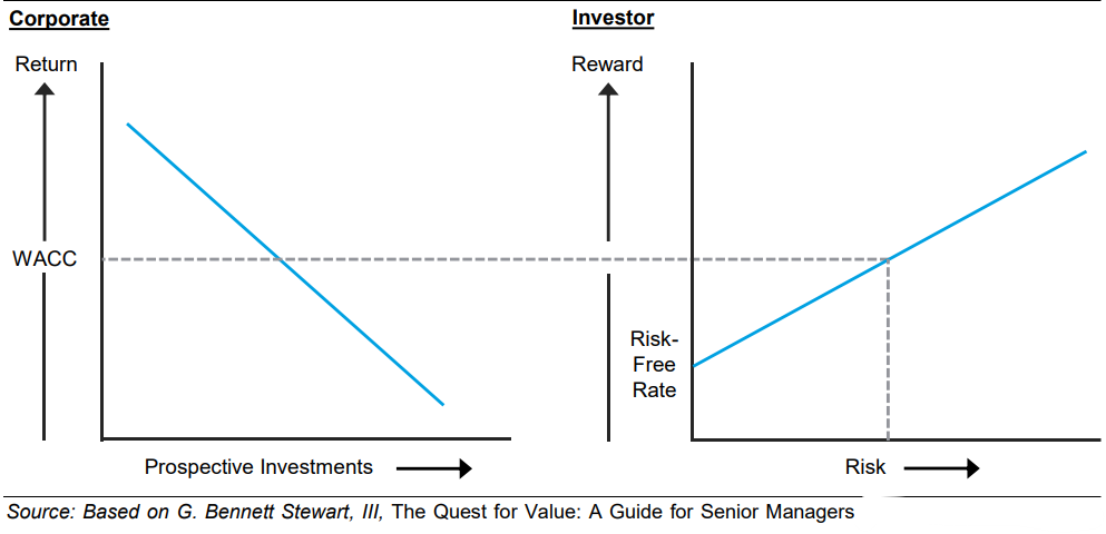
The cost of capital links corporate finance to investing; companies use the capital that investors save, ideally at a rate of return above the cost of capital (i.e. the opportunity cost of that capital) in order to create value for those investors. These capital allocation decisions apply to M&A, R&D, and other internal investments and capital expenditures. Typically, mature companies can only invest so much before the return on investment drops below the cost of capital, at which point they ought to return excess cash flows directly to shareholders.

Leverage and Capital Structure

Business risk describes the variability of operating cash flows. The term is often interchangeable with operating leverage, which measures changes in operating profit per percent changes in sales. The ratio of fixed to variable operating costs is a determinant of operating leverage: firms with high fixed and low variable costs have more operating leverage than those with low fixed and high variable costs. The astute reader may note that financing via high amounts of debt synthetically creates operational leverage by increasing fixed costs (i.e. interest payments) and therefore makes earnings more volatile.

We claim that companies with high business risk would want to have low financial risk while shareholders of companies with low business risk benefit from having some financial risk. This may seem intuitive, but its useful to recap the theory.

We first note that by the Modigliani–Miller theorem, under the assumptions of no taxation, no transaction costs, and uniform borrowing rates, the enterprise value of a firm is independent of its capital structure. That is to say, a change in the capital structure under these assumptions does not generate value, and does not change risk for the firm but rather simply transfers risk from one stakeholder to another.

In particular, the cost of debt also goes up when a company adds debt but the cost of equity also goes up because equity is the return on the residual claim, which is now riskier. But the overall weighted average cost of capital (WACC) is the same since debt is less costly than equity due to its seniority in the capital structure. Under these assumptions, the returns on the two financing methods are given by

r_E = r_0 + \frac{D}{E}(r_0 - r_D)

Where rE is the expected rate of return on equity of a leveraged firm, r0 is the company cost of equity capital with no leverage, rD is the expected rate of return on borrowings, or cost of debt, and D/E is the debt-to-equity ratio.

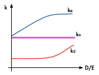
Assuming that the cost of each asset class (k) is equal to their returns, we note that the weighted average cost of capital (k0) remains constant even as cost of equity (ke) and cost of debt (kd) changes. As such, the value of the unlevered firm (Vu) and the value of the levered firm (Vl) are the same since their future cash flows are discounted by the same weighted average cost of capital.

These results might seem irrelevant (none of the conditions are met in the real world), but the theorem is important precisely because it tells us where to look for determinants of optimal capital structure when its assumptions are violated. In particular, most jurisdictions treat interest expense as a deduction from income before paying taxes, while dividend payments are not deductible. That means debt adds value to the firm because more cash flow is going to stakeholders and less is going to the government.

Assuming that the firm’s debt is funded by perpetual bonds (akin to equity being a perpetual variable claim) under fixed and known interest rates, then we know that the amount of annual interest is given by Debt x Interest Rate. The Annual Tax Shield is therefore equal to Debt x Interest Rate x Tax Rate. The perpetual value of this annual tax shied is discounted by the same interest rate, and so is equal to Debt x Tax Rate. In short, for a corporate tax rate of T and debt value of D, the debt financing adds DT to the enterprise value of the firm. Assuming the business has no risk, then it is beneficial to finance the entire operation with debt since it means that the corporation can avoid paying taxes entirely if its EBIT is equal to its interest. The return on equity is given by the following

r_E = r_0 + \frac{D}{E}(r_0 - r_D)(1-T)

In the real world, business risk exists. A company’s optimal capital structure therefore is determined by the trade-off between the financial benefits of debt and the risk of financial distress that maximizes the value of the firm. As a company adds debt the benefit of the tax shield initially rises at a rate faster than the cost of financial distress (almost minimal in the absence of initial debt); however, at some point, the cost of financial distress exceeds the benefit of the tax shield. Why is this the case? One way to think about it is that shareholders are no longer able to enjoy the benefits of the interest tax shield if the company ever becomes bankrupt. As such, increases in the probability of default reduces the value of the tax shield.

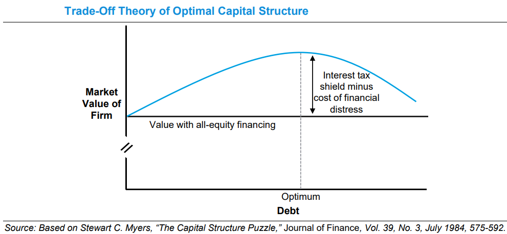
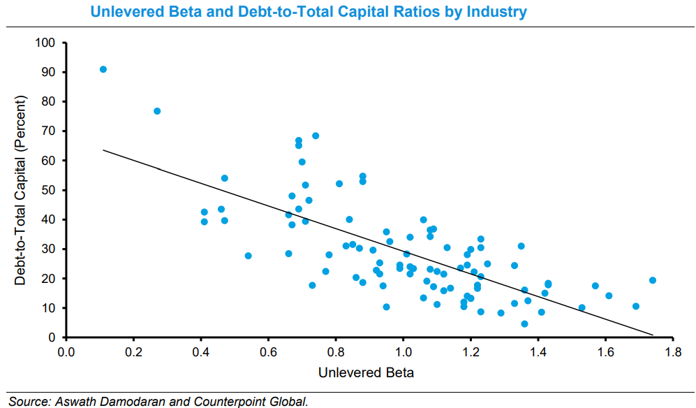
Therefore, companies with high business risk would not benefit from the tax shield as much while shareholders of companies with low business risk benefit greatly from the tax shield. We confirm this empirically by inspecting the relationship between the undiversifiable business risk (measured with unlevered beta i.e. exposure of operating profits to the macroeconomic environment in a 1-factor model) and the ratio of debt to total capital of the firm:

The theory also helps explain the rise of the leveraged buyout industry from the 60s to the 80s (A LBO is a transaction where a financial sponsor buys a company that has stable cash flows and finances the deal with a high debt); the rise of leveraged buyouts coincided roughly with the period in US history which saw some of the highest levels of corporate taxation. As such, loading up otherwise stable companies with debt may have increased their risk, but also generated tremendous shareholder value by removing the portion of the government’s claim.

In recent times, especially since the GFC, firms have typically been conservative with the amount of leverage they take on. This is probably explained by a combination of factors. First, while the US tax code still favors debt over equity financing, both the effective and statutory tax rate for corporations have never been lower.

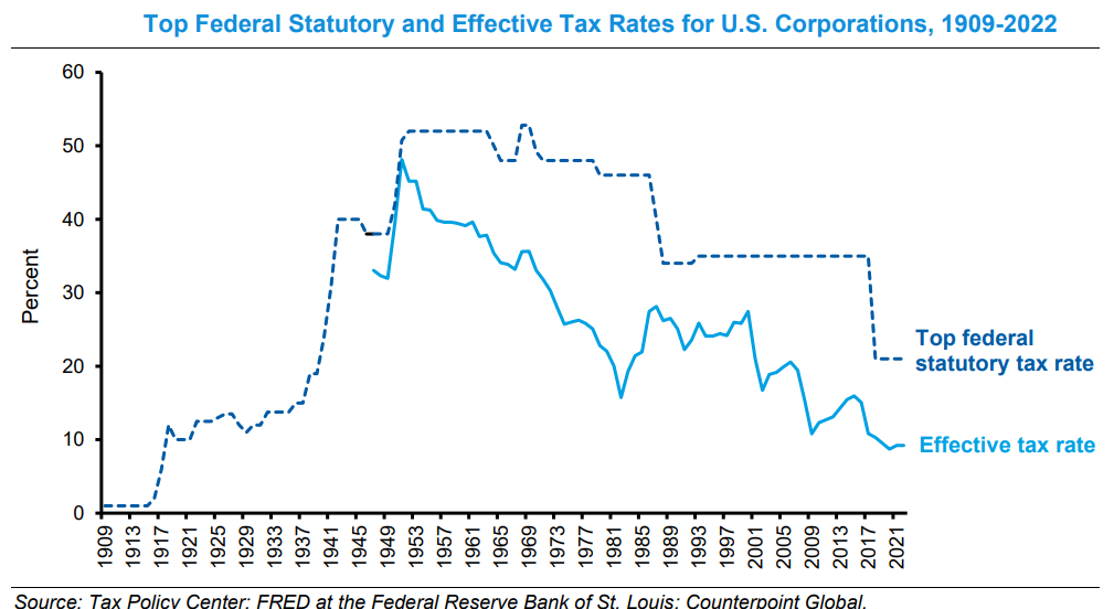
The low effective tax rate of American companies reduce the need for the tax shield provided by leverage. Part of the reduction in corporate taxes can be explained by legislation (see dotted line for the top statutory rate), but another part can also be explained by skillful corporate accounting. For example, we note that the operations of large American companies have become more global over time, and that global presence provides them with the opportunity to manage where their profits are taxed.

In addition, the fact that many modern sectors focus on intangible investment also offer tax benefits. We note that companies expense intangible investments on their income statement and therefore reduce pre-tax profit immediately; on the other hand, companies capitalize tangible investments, which means they record them on the balance sheet and depreciate them on the income statement over the asset’s estimated useful life, meaning that the tax benefit is spread out (typically linearly). However, we know that the present value of a deduction is greater than its future value, which means that an intangible and tangible investment of the same magnitude and payback implies a higher tax-adjusted value of the intangible investment.

In short, we have shown that the optimal capital structure exists partially because of tax reasons, and balances the benefits of the tax shield against increased risk. In addition, the particular capital structure of a firm creates two assets (stock and bond) with different risk-return characteristics partially determined by the financial leverage of the firm. Firms with low business risk should prefer leverage while those with high business risks should avoid it. Large corporations that can benefit from other tax shields or those in jurisdictions with low corporate tax rates naturally derive less benefits from leverage.

The Cost of Debt

The cost of debt is the effective after-tax rate a company has to pay on its [long-term] debt. For companies rated investment grade, the yield to maturity on long-term bonds is a good estimate for the pre-tax cost of debt and can be observed directly.

The focus on the use of long-term debt stems from the fact that the time horizon for estimating the cost of capital should match the time horizon of forecasted cash flows, which is rarely less than ten years. However, if we are trying to calculate the net present value of a project that is only expected to generate cashflow for the next five years, it would technically be appropriate to use short-term yields for cost of capital calculations. Additionally, we note that the long-term rate is a better approximation of interest costs over time even for companies that roll over their short-term debt because long-term rates capture the expected cost of repeated borrowing. If a company exclusively relies on short-term debt, has highly illiquid debt, or mostly has debt with embedded optionality, we can use its credit rating to approximate the cost of long-term debt without optionality.

Technically, for non-zero probability of default, the yield to maturity overestimates the cost of debt since in the case of restructuring / liquidation, the company does not need to keep paying its debt holders the originally agreed-upon interest, and this results in a lower expected cost of debt. However, for investment grade bonds this bias is small enough as to not need a correction. To see why, consider the case of a zero-coupon bond rated investment grade; it has fair value

V = F \cdot (1-p) \cdot e^{-YT} + F \cdot p \cdot R \cdot e^{-rT}

Where Y is the yield to maturity, r is the risk-free rate, T is the time to maturity, V is the present value of the bond, F is the promised future payment, p is the probability of default and R is the recovery rate. For small p, the right term vanishes and leaves us with the value of the bond approximately equal to the left term alone. Now, a natural question to ask is: “why does the probability of default not matter in the above calculation, but still matters in causing Y to be greater than r?” i.e. how do we now justify that investment grade returns need to be substantially higher than risk-free returns even for very small probabilities of default over long horizons?

We can answer this question by considering the relationship between p, Y, and r. Consider a substitution of V by the fair price of the bond

F \cdot e^{-YT} = F \cdot (1-p) \cdot e^{-rT} + F \cdot p \cdot R \cdot e^{-rT}

Divide by F, take the natural log, and simplifying, we get

Y = r - \frac{1}{T} \ln(1 - p(1-R))

Since ln(1 - p + pR) < 0 for 0 < p < 1 and R < 1, we can see that Y > r. Moreover, recall that the graph of -x is always above the graph of ln(1-x) (which tend toward negative infinity at x = -1) due to the convexity of the exponential function. In other words, as a consequence of Jensen’s Inequality, p has a much greater effect on Y than we’d otherwise expect.

To capture the value of the tax shield in our cost of capital calculations, we must adjust debt from a pre-tax rate to an after-tax rate. To do this, we multiply the pre-tax cost of debt by one minus the marginal tax rate - the tax rate a company pays on its last dollar of taxable income. This calculation is often done using the federal statutory tax rate in more elementary models, but this overestimates the value of the tax shield since we saw in the previous section that most firms pay an effective rate of around half the statutory rate.

The calculation for the value of the tax shield is non-trivial and is complicated by the complexity of tax legislation. For example, not all companies can take all of their interest expense as a deduction from taxes; starting in 2022 the tax deductibility of interest was capped at 30% of EBIT for U.S. companies with sales of $25 million+. We must also note that the effective rate is also commonly much lower than the marginal rate because companies have net operating losses, tax loss carrybacks, investment tax credits, and tax avoidance strategies that do not affect the rate paid on the last dollar of taxable income. In this post we do not seek to discuss all of the intricacies of how firms optimize tax efficiency, but merely to show that the complexity of the tax code can make an accurate calculation of the tax shield difficult.

After accounting for the value of the tax shield, we arrive at the cost of debt. We now show the long-run cost of debt for investment grade firms below:

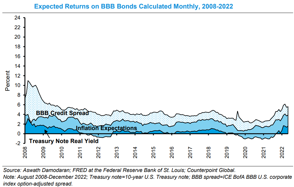
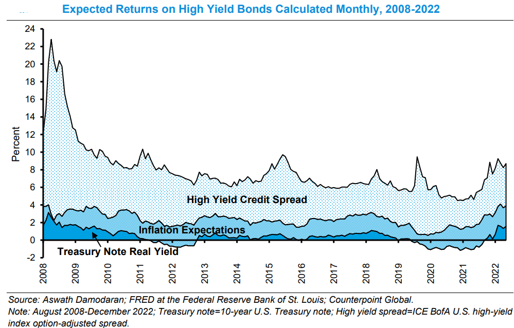
Yield to maturity overstates the pre-tax cost of debt for companies issuing high-yield debt since high-yield bonds have a meaningful probability of default (10 years default rate is about 2% for an investment-grade bond and 20% for high-yield). In general, we know that Cost of debt = promised yield spread – lost yield due to default. For high-yield bonds, the true cost of debt is somewhere between the promised yield and investment grade yield. The process for estimating this true cost is a bit involved so we will skip it for now (potential subject for future post).

In addition to bonds, we note that all types of liabilities in theory should be accounted for in calculating the cost of debt. Long-term leases, for example, should also be considered debt since they oblige periodic payments in return for an asset (the right of use of the facility); the cost of a lease, however, reflects in part the return on capital of the landlord’s investment and as such can be substantially different from the cost of debt of the tenant. In general, substantial holdings of non-bond liabilities make it challenging to evaluate a firm’s true cost of debt.

The Cost of Equity and CAPM

The cost of equity is the total return that can be expected in a competitive market given the risk profile of the firm. The cost of equity should be higher than the cost of debt because it represents a subordinate claim; this gives us a lower bound. Otherwise, estimating the cost of equity is challenging because it cannot be directly observed. In contrast, when a company issues debt, the cost is relatively clear.

As such, calculating the cost of equity typically requires the use of asset-pricing models, the most well-known of which is the Capital Asset Pricing Model (CAPM). In theory, it would be appropriate to use multi-factor models that consider style risks such as momentum, size, value, etc… However, the CAPM is often used in practice due to its simplicity and because estimates of factor risks are noisy.

The Capital Asset Pricing Model (CAPM) calculates the expected return of a security by adding the risk-free rate to the product of the security’s beta (β) and the equity risk premium (ERP). In this model, the ERP represents the difference between the expected return of the overall market and the risk-free rate. Since the CAPM assumes that only systematic risk—risk that cannot be diversified away—affects excess returns, the ERP is the same for all stocks.

To clarify, systematic risk refers to broad market risks that affect all investments, such as changes in interest rates or economic conditions. Because investors cannot eliminate these risks through diversification, they demand compensation for bearing them. Beta (β) measures how sensitive a stock is to these market-wide risks, with a higher beta indicating greater sensitivity and higher expected return.

On the other hand, risks specific to individual companies or industries—known as diversifiable risks—can be mitigated by holding a well-diversified portfolio. In an optimal portfolio, these diversifiable risks would essentially be eliminated. As a result, investors do not expect to be compensated for these risks, which is why only systematic risk, captured by beta, influences the expected return.

r_i = r_f + \beta_i (r_m - r_f)

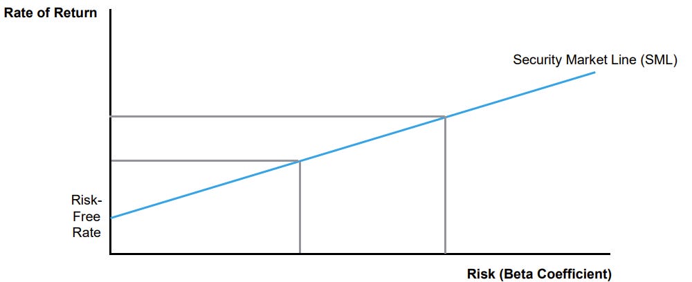
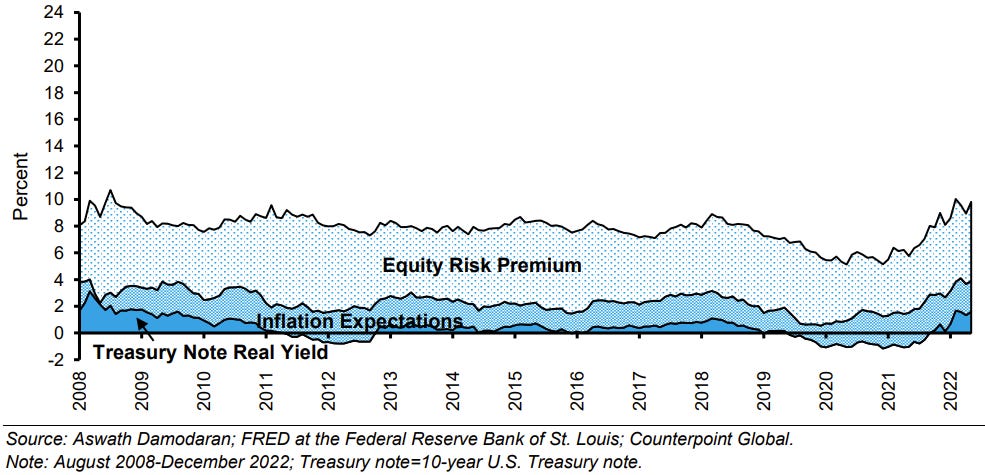
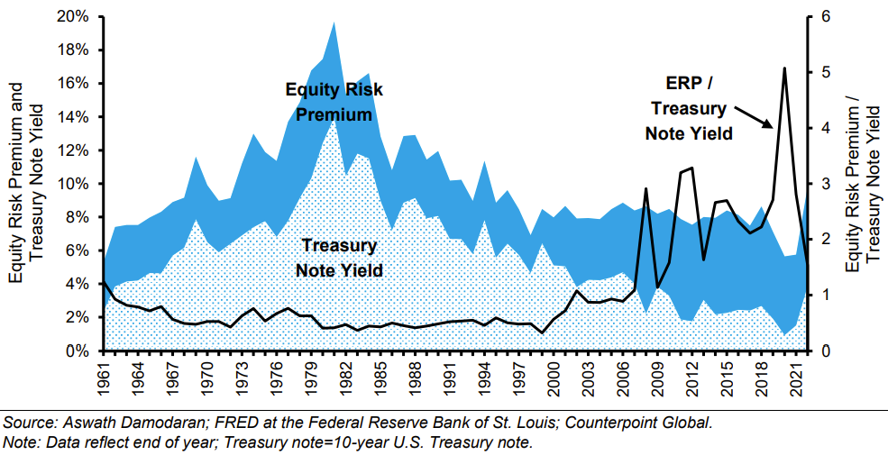
While the CAPM presents an elegant theory, it is difficult to use in practice. Of the components in its equation, only the risk-free rate is directly observable via treasuries. The Equity Risk Premium (ERP), on the other hand, is easy to observe historically but difficult to predict (as it should be, since predicting the ERP would be equivalent to predicting stock returns). Typically it is believed that the long-run ERP is between 3 to 10 percent. Determinants of the ERP include macroeconomic / productivity growth, collective risk aversion, the perceived level of economic risk, the degree of liquidity in markets, the tax policy, et cetera; ERP is probably not a stationary time-series.

Equity Risk Premium

Instead of building sophisticated models, the most common approaches to estimating the ERP are (1) to look at historical results and assume the future will be similar (2) to survey investors about their expectations and (3) to estimate a rate the market implies (via P/E Ratios) by reverse-engineering assumptions to solve for the market price.

Each method is imperfect; historical results are highly sensitive to the time period selected; survey results are highly variable depending on the sampling method, phrasing of questions, and animal spirits; and an ERP implied by the market uses current prices but requires assumptions for inputs such as cash flow growth. While estimates of 10-year ERPs by economists are noisy, they do appear to be much better than randomly guessing. See consensus estimates vs realized below:

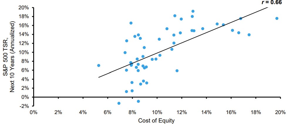
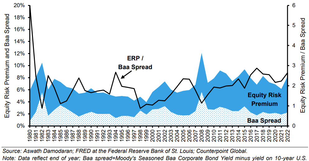
Comparing the ERP to credit spreads is another way to assess whether it is calibrated sensibly. Periods of very high valuations in the equity markets therefore imply low future equity returns. The peak of the market in March 2000 is an example where valuations were high and as such returns for large cap stocks were predictably poor for the following decade. Note, however, that simply knowing returns will be poor for the next decade doesn’t tell you whether you should buy or sell now, since it may well be the case that the bubble will double or quadruple before it pops.

Beta

The last term to estimate before getting the cost of capital is the beta of the stock. It is well known that beta as it is understood in CAPM has several problems, the largest of which is that it is highly unstable and therefore often fails to predict returns. Nonetheless, the historical beta (obtained via a regression analysis with the market’s total returns) is typically the starting point for estimating beta. See Nike below:

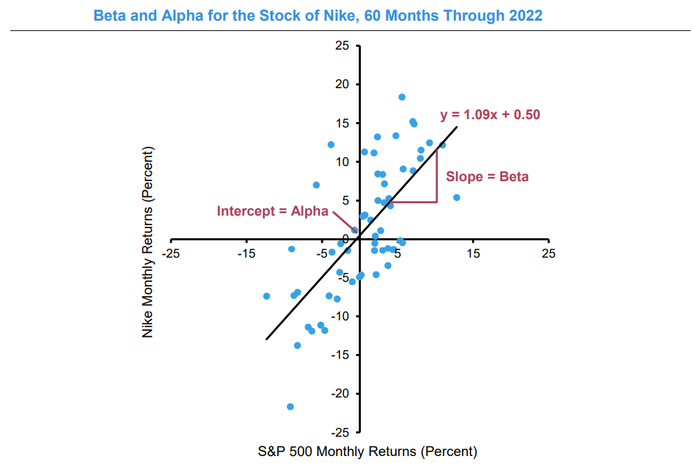
There are a few decisions to make when estimating historical beta. The simplest is the benchmark used for the estimate (use the S&P 500), and more complicated decisions include the length of the lookback period and the frequency of sampling. The benefit of going back further is that there are more data but the drawback is that the company may have changed its business model or have simply matured in its space; more frequent measurement creates more data, but potentially exposes the estimate to effects of outliers (kurtosis of 1-day returns much higher than 10-year returns).

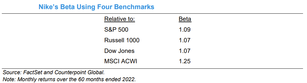
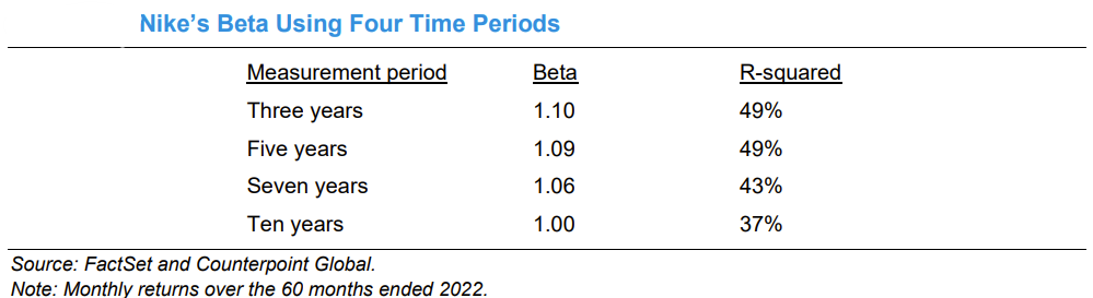
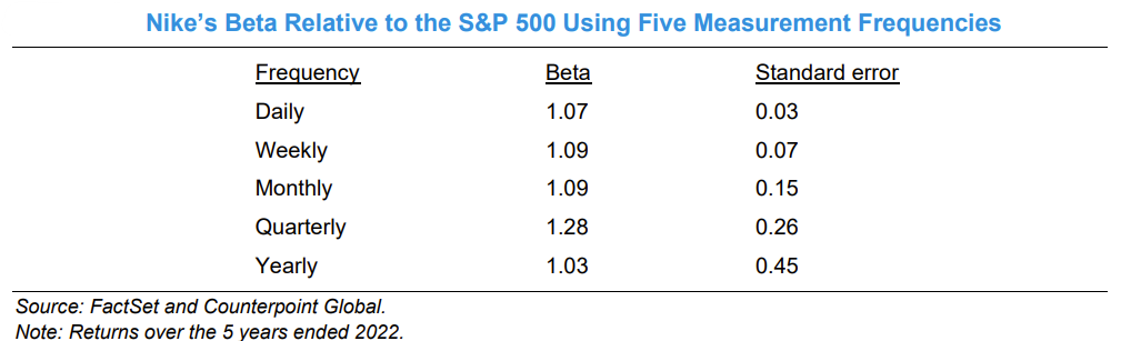
Given large standard errors relative to the size of estimate, practitioners have developed some tricks to reduce the MSE of estimates. First, assuming that financial leverage increases beta linearly, we can estimate the unlevered beta of the firm which captures only its business risk and not its financial risk. The estimate for the unlevered beta can then be re-levered for the current level of financial leverage.

Regularization can also help; knowing that the capitalization-weighted beta of the market is 1, we can do a weighted average between the estimate of beta and 1; Bloomberg’s adjusted beta only uses 2/3 of the raw beta. Additionally, using sector beta can also help reduce the variance of the beta estimate. While regularized estimates introduce bias, it is not unreasonable to think that the variance reduction is probably greater.

Weighted Average Cost of Capital

The weighted average cost of capital (WACC) combines the opportunity cost of the sources of capital with the relative contribution of those sources. The weighted average cost of capital is therefore the appropriate rate at which to discount the future free cash flows attributable to the firm to determine their present value. It should be noted that when discounting cash flows attributable to equity holders only, it is appropriate to discount using the cost of equity.

To elaborate, WACC represents the required return that investors expect for providing capital to a firm, considering the mix of debt and equity the company uses. In an efficient market, where investors could allocate their capital to other investments with similar risk profiles, WACC serves as the opportunity cost of capital. This means that when we discount future cash flows, WACC ensures that we account for the return investors could have earned elsewhere.

In competitive markets, investors are assumed to hold diversified portfolios, which means they are concerned primarily with systematic risks—those that cannot be diversified away. Since WACC incorporates the cost of equity (which reflects systematic risk) and the cost of debt (which accounts for tax shields), it accurately reflects the expected return in such a market. Diversifiable risks specific to the company are not priced into WACC because a diversified investor would have eliminated them.

There are not a lot of decisions to make when calculating WACC assuming you have the cost of debt and cost of equity. The only point worth noting is that the weighting of debt and equity should be based on market values and not book values. The reason is that opportunity cost is based on the prevailing asset price rather than the level at which the company reflects debt or equity on the balance sheet.

Capital Structures Evolving

In a programmable‐finance world, capital claims no longer sit neatly at the poles of debt and equity. Instead, every economic right—from revenue shares to governance votes—can be unbundled and recast as on-chain tokens. A protocol might issue pari passu coins that mirror common equity, or layer senior and subordinated tranches so that Token A pockets the first slice of fees and Token B only what remains. Hybrid structures—tokens that pay a modest “coupon” and then convert into upside-participation units—become trivial to code, eliminating the need for legal wrappers.

Minting schedules, too, transform into programmable curves rather than contractual covenants. You could cap supply at 21 million, mint new tokens at a constant linear rate, taper inflation via a tail-emission, or trigger issuance only when on-chain milestones (TVL thresholds, governance quorum) are hit. Because these rules live in immutable smart contracts, protocol designers can fine-tune incentives—rewarding early adopters, sustaining security, or stabilizing value—simply by adjusting parameters in code instead of renegotiating indentures.

To estimate each tranche’s “cost of coin,” we can adapt familiar valuation tools to the blockchain. First, forecast on-chain cash flows—fee dividends, staking rewards, rebases or burns—according to the token’s emission and waterfall logic. Next, layer in risk adjustments for seniority spreads (the extra yield junior tokens demand), smart-contract and oracle vulnerabilities, and each coin’s sensitivity (“beta”) to a broader crypto index. Finally, choose your discount framework: a crypto-CAPM (stablecoin lending rate plus beta × crypto risk-premium), a tranche-level IRR solved via simple scenario analysis, or an implied yield back-solved from secondary‐market prices and the emission curve.

Ultimately, programmable finance recasts capital structure as a living organism rather than a static trade-off. Protocols can recalibrate risk–return slices in real time, align incentives across engineers and investors, and even automate capital-structure arbitrage—all through on-chain code. But this newfound flexibility also challenges our classical frameworks and forces regulators, accountants, and practitioners to rethink what “debt,” “equity,” and “worth” mean when every attribute of claim becomes programmable.