The Effects of Spot-Vol Correlation

From The Logbook. The original article is reproduced in full, with minor grammar corrections; references to market conditions reflect the context in which it was written.

Skew and smile in option prices can be interpreted through the lens of local volatility, which reflects the variability of volatility at different strikes. This suggests that volatility is not constant but depends on the underlying asset's price, a behavior that can be linked to the correlation between the spot price and its volatility (e.g., VIX ticks down when S&P 500 ticks up). This dynamic also implies that volatility exposure (vega) can be hedged using delta adjustments, as the movement in the underlying directly influences volatility. Additionally, because different deltas imply different levels of gamma, the value of the option is impacted. We reference chapter 7 of Trading Volatility.

Moving the Vol Curve

It is well known that the implied volatility (IV) of options across strike is not constant and that smile (the tendency for OTM options to have higher IV), skew (the tendency for the downside / upside to have higher IV), and term structure (the tendency for front / back options to have higher IV) exist due to many various market dynamics, investor preferences, and fundamental characteristics of underlying assets.

For example, higher IVs for deep OTMs may exist because empirical returns are not normally distributed but have fatter tails, and higher IVs for mid-range OTMs may exist due to vol of vol exposure. Skew may exist with the downside being more expensive because of either investor demand buying puts for crash protection, or covered-call ETFs systematically selling calls, or both.

A natural question which arises when the spot moves is how we should shift the vol curve. Naively, we may be tempted to simply shift it so that the vol of the x delta option post spot ticking is the same as the vol of the x delta option prior to spot ticking (this model is intuitively called “sticky delta”). See visualization below:

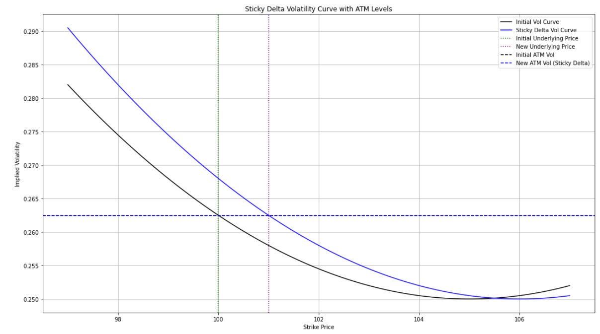
Note that post shift, the ATM vol remains the same as before (as intended), but the vol of the option at the previous ATM strike has gone up, which seems somewhat unintuitive. Moreover, we know that empirically returns are negatively correlated with vol (steady slow uptick gives the lower vol) and we feel that the way we shift our vol curve should reflect that fact. So perhaps we shift the new ATM vol down and assume that dσ/dS = dσ/dK (i.e., we move vol down according to the ATM slope). Because the vol curve is locally linear, the strike vol on each strike stays roughly the same (this model is intuitively called “sticky strike”). See visualization below:

Another way to think about sticky strike is as a stable (or unmoving) volatility surface that the spot moves along. For a put skew, a sticky strike model implied negative correlation between spot and vol. On the other hand, sticky delta assumes a constant volatility for options of the same strike as a percentage of spot and therefore implies there is a positive correlation between volatility and spot.

Is sticky strike a correct model? Unfortunately the answer is no. For example, consider AMZN 2018-04-26 pre earnings front vol curve:

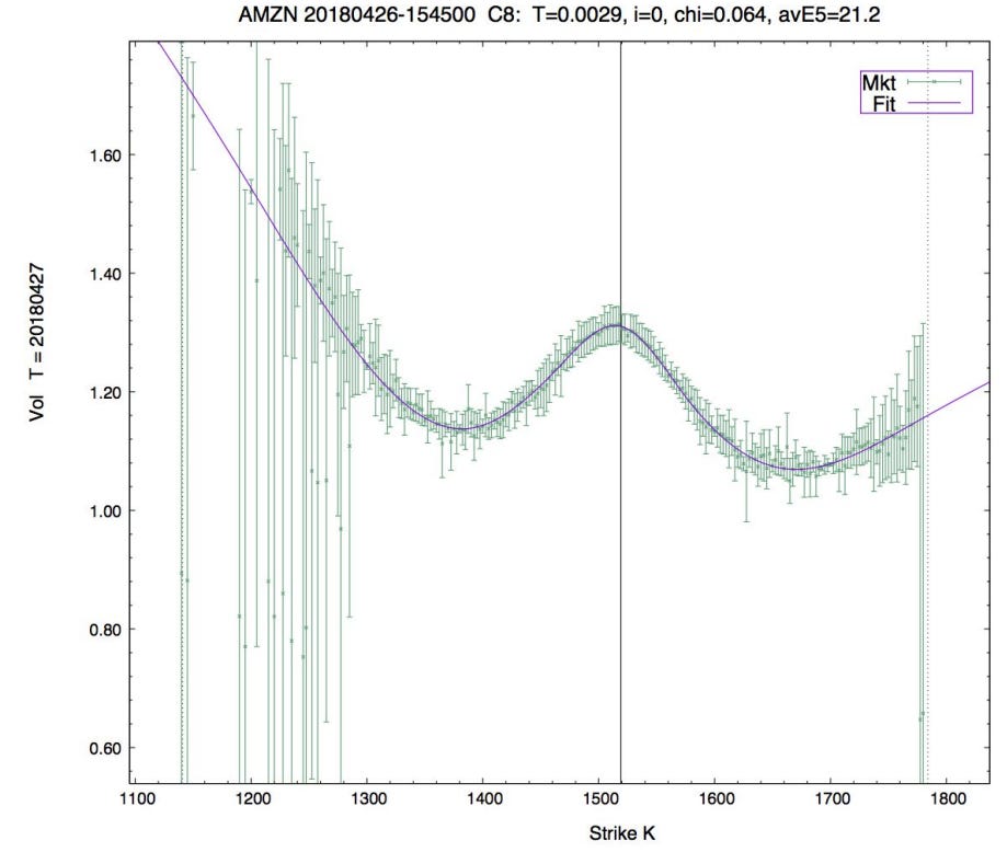
Note that the slope ATM is actually 0 since the bimodal earnings event has distorted the vol curve into a W shape (the exact reasons for this can be discussed in another post). Does this mean that the spot-vol correlation is 0? Of course not! We know that the vol curve is distorted by an event and what we really want is to take out the event to get what the “natural” vol curve would look like without the event:

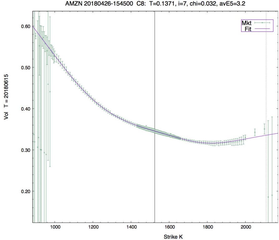
Can we then use the vol curve after taking out events (or vol curves in the absence of events) to determine how much vol should move with spot (i.e. the spot-vol corr)? Unfortunately, the answer is probably still no, for a few reasons: (1) our natural slope is entirely determined by how we model the event (2) the natural slope itself can be dislocated due to flow (3) there is no fundamental reason for dσ/dS = dσ/dK to hold.

In fact, using dσ/dK to price dσ/dS is like using IV to price RV. Just as how we would rather know how vol is going to realize and trade implied, we’d rather know what corr spot and vol will realize and express that opinion on skew. Moreover, the strike vol’s correct interpretation is probability-weighted average vol of all possible paths from the spot that crosses the strike, and hence the actual change in vol with respect to spot is almost surely higher than the change in vol with respect to strike (assuming the strike not at the money has higher vol).

In the absence of a strong opinion on spot-vol corr we can fit to market, but even in this case neither sticky delta nor sticky strike is always “correct.” For example, while a variant of running negative spot-vol correlation is typically a decent fit, one can imagine a counterexample in a stock that has been continuously up-ticking: it will reach some very low vol, but then there is a fundamental level of vol that the market will not go below, at which point the curve behavior will start to resemble sticky delta.

Indeed, IV is just a social construct. It is investor sentiment that determines which implied volatility / spot-vol correlation regime the market trades in.

Adjusting the Delta

How a volatility surface reacts to a change in spot changes the value of the delta (dV/dS) of the option. If there is no spot-vol correlation, then the total derivative of the value of the option with respect to spot dV/dS is equal to the partial derivative ∂V/∂S. However, if there is dependency between spot and vol, we can apply the chain rule

\frac{dV}{dS} = \frac{\partial V}{\partial S} + \frac{\partial V}{\partial \sigma}\frac{\partial \sigma}{\partial S} = \Delta_{BS} + \nu \rho

We see that true delta (also known as the skew delta or shadow delta) is equal to the Black-Scholes delta plus a second term that is the product of the option vega and the derivative of the vol with respect to spot. If this derivative is negative, then the skew delta will be less than the Black-Scholes delta. Intuitively this makes sense if we consider the value of a call as spot moves up: the call gains value from Black-Scholes delta exposure but loses value from vega since now vol is lower.

The effect of skew on delta affects the way to optimally hedge a option’s exposure. Because spot is correlated with vol, part of the vol exposure of an option is captured in its delta and can be hedged away with the underlying. The discerning reader will also quickly note that spot-vol correlation will likely have direct impacts on the gamma of the option, since gamma is just the derivative of delta with respect to spot. Since the value of the option is equal to the amount we can expect from gamma scalping, it follows that skew also affects not only our hedging, but the value of the option itself.

Trading Skew

If an investor initiates a long skew position by buying an OTM put and selling an OTM call, the implied volatility of the put purchased has a higher implied volatility than the implied volatility sold through the call. The long skew position therefore has a cost associated with it, which is typically called the ‘skew theta’.

Our typical understanding of theta is that it is the cost associated with gamma and that at fair value nets to the risk-free rate of return over the lifetime of the option; similarly, skew theta can be interpreted as the cost associated with gaining exposure to the correlation between spot and vol.

A long skew trade profits from negative spot volatility correlation. For example, let us assume an investor is long skew by long an OTM put and short an OTM call: if equity markets decline, the put becomes ATM and is the primary driver of value for the position (as the OTM call becomes further OTM it is far less significant). The rise in the volatility surface (due to negative correlation between spot and volatility) boosts the value of the (now ATM) put and, hence, the value of the position.

A long / short skew trade breaks even if the local volatility surface stays constant. We can see this since the amount volatility surfaces move for a change in spot is equal to the skew and this movement is exactly the correct amount for the profit (or loss) on a volatility surface re-mark to compensate for the cost (or benefit) of skew theta. Therefore, a long skew trade profits when spot-vol correlation is more negative than what strike-vol slope suggests, and vice versa loses money when spot-vol correlation is less negative than what strike-vol slope suggests.

The relationship between skew and gamma is closer than one would initially think; it is in fact possible to show mathematically the relationship between skew trading and gamma trading if one assumes a correlation between spot and volatility. To see how this is the case, we first note that Vanna (dVega/dSpot) can be used as a measure of the size of a skew position. This can be seen intuitively from the argument that as markets decline the primary driver of value in a skew trade is the change in vega (long put dominating the short call) for a change in spot.

Note now that Vanna = dVega/dSpot = dDelta/dVol, and since Vol ~ Spot

Vanna ~ dDelta/dSpot, and since Gamma = dDelta/dSpot

Vanna ~ Gamma

Therefore, Vanna trade can be considered to gamma trading due to the negative correlation between volatility and spot.

Recap

The concepts of skew, smile, and term structure in option pricing arise from the fact that implied volatility (IV) is not constant but varies across strike prices, maturities, and market conditions. Spot-vol correlation complicates volatility hedging and impacts option pricing, as delta adjustments can capture some vega exposure, influencing gamma and, therefore, the value of options via gamma scalping.

The interaction between spot-vol correlation and option pricing highlights key differences between regimes like "sticky strike" and "sticky delta." Neither model perfectly captures reality, as empirical vol behavior often deviates due to flow, market dynamics, or fundamental limits on volatility.

Skew trading profits or loses based on deviations between actual spot-vol correlation and the slope of the vol curve. Ultimately, skew positions, through vanna (dVega/dSpot), closely relate to gamma trading i.e. IV-RV trading.