The Equity Risk Premium Puzzle

From The Logbook. The original article is reproduced in full, with minor grammar corrections; references to market conditions reflect the context in which it was written.

Between 1889 and 1978, the average real return on U.S. equities (S&P 500) was 6.98% per year. The average real return on short-term government debt was 0.80%. The difference — 6.18 percentage points — is the equity risk premium. That spread is large. But the puzzle isn’t the number itself. The puzzle is that standard economic theory, under any reasonable assumptions about human behavior, cannot generate it.

Two Assets, One Consumer

In 1985, Rajnish Mehra and Edward Prescott published “The Equity Premium: A Puzzle” in the Journal of Monetary Economics. They set up the simplest possible representative-agent economy: There is a single representative consumer who lives forever, consumes a single perishable good each period, and can trade two assets: a risk-free bond and a risky equity claim. The consumer maximizes the expected present value of lifetime utility:

\max \; E_0 \left[ \sum_{t=0}^{\infty} \beta^t \, u(c_t) \right]

where β ∈ (0,1) is the subjective discount factor (how much the consumer discounts future utility relative to today), and u(·) is a strictly increasing concave utility function. In this case they use constant relative risk aversion (CRRA) preferences:

u(c) = \frac{c^{1-\gamma}}{1-\gamma}

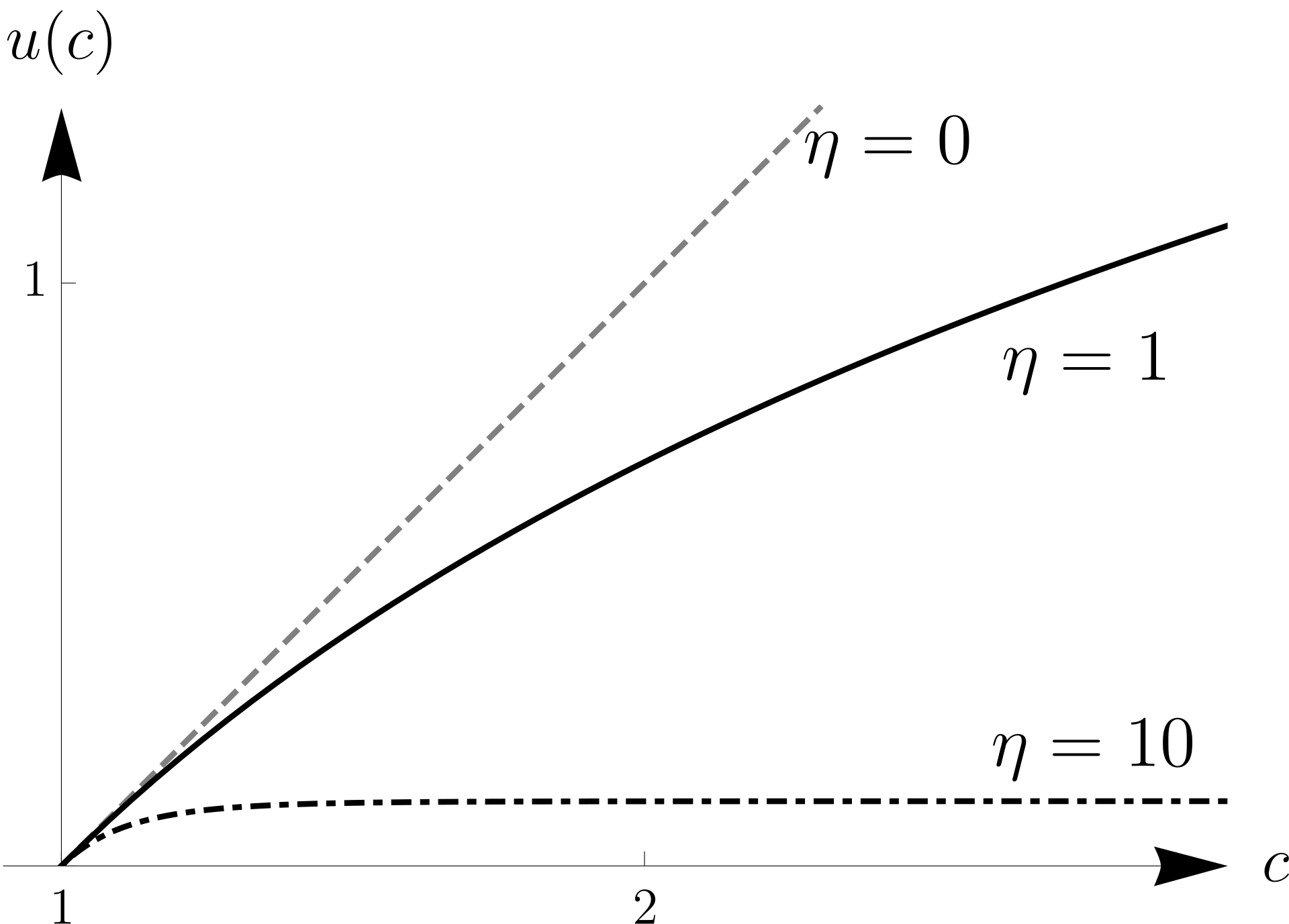
(When γ = 1, this collapses to u(c) = ln(c) by L’Hôpital’s rule.) The single parameter γ is the coefficient of relative risk aversion. It governs how much the consumer dislikes uncertainty in consumption. Formally:

\gamma = -c \frac{ \, u''(c)}{u'(c)}

γ is therefore the curvature of the utility function, scaled by the level of consumption so that it’s unit-free. Higher γ means the marginal utility of consumption falls off faster as consumption rises, which means the consumer cares more about avoiding bad states relative to reaching good ones.

Under CRRA, γ also equals 1/ψ, where ψ is the elasticity of intertemporal substitution (EIS), i.e. how willing the consumer is to shift consumption across time in response to interest rate changes. This dual role is important: it means a single parameter controls both risk aversion and inter-temporal substitution

The Euler Equation & Stochastic Discount Factor

The consumer faces a budget constraint each period and chooses how much to consume vs. invest. For any asset i with gross return Rᵢ,ₜ₊₁, the first-order condition of the maximization problem is:

u'(c_t) = \beta \, E_t \left[ u'(c_{t+1}) \, R_{i,t+1} \right]

This is the Euler equation. The intuition is marginal: at the optimum, the consumer is indifferent between consuming one more unit today (gaining u’(cₜ) in marginal utility) and saving that unit, earning return Rᵢ,ₜ₊₁, and consuming the proceeds tomorrow (gaining β u’(cₜ₊₁) Rᵢ,ₜ₊₁ in expected discounted marginal utility). If one side were larger, the consumer would adjust, so at the optimum, they’re equal.

Dividing both sides by u’(cₜ) and define the stochastic discount factor Mₜ₊₁,

1 = E_t \left[ \beta \, \frac{u'(c_{t+1})}{u'(c_t)} \, R_{i,t+1} \right]

m_{t+1} \equiv \beta \, \frac{u'(c_{t+1})}{u'(c_t)}

Mₜ₊₁ can also be interpreted as the marginal rate of substitution. The Euler then naturally equation becomes:

1 = E_t \left[ m_{t+1} \, R_{i,t+1} \right]

This single equation prices every asset in the economy. It says: the expected product of the SDF and any asset’s gross return equals one.

We can think of mₜ₊₁ as the exchange rate between dollars today and dollars in state s tomorrow, measured in utility units. It answers: how much is a dollar delivered tomorrow in state s worth to me today, relative to a dollar right now?

- When cₜ₊₁ is low (bad state), marginal utility u’(cₜ₊₁) is high, so mₜ₊₁ is high. A dollar in the bad state is very valuable, as the consumer is desperate for wealth / consumption.

- When cₜ₊₁ is high (good state), marginal utility is low, so mₜ₊₁ is low. A dollar in the good state is less valuable, as the consumer is already well-fed.

An asset that pays off well when m is high (i.e., in bad states) is like insurance, it’s valuable, so the market bids up its price, and its expected return is low. An asset that pays off well when m is low (good states), like equities, which boom when the economy booms, is the opposite of insurance. The market pays less for it, and it must offer a higher expected return to compensate. That’s the equity risk premium.

Under CRRA utility, the SDF has a concrete form

m_{t+1} = \beta \left( \frac{c_{t+1}}{c_t} \right)^{-\gamma}

The SDF is the discount factor β times consumption growth raised to the power −γ. When consumption growth is high, m is low (good times are cheap). When consumption growth is low or negative, m is high (bad times are expensive). The parameter γ controls how sensitive this exchange rate is to consumption fluctuations.

Pricing the Risk-Free Bond

Apply the Euler equation to a risk-free asset with known gross return Rf

1 = E_t \left[ m_{t+1} \, R_f \right] = R_f \, E_t[m_{t+1}]

Since Rf is known at time t, it comes out of the expectation. Solving

R_f = \frac{1}{E[m]}

The risk-free rate is the inverse of the expected SDF. When the consumer is patient and expects wealth to grow slowly, E[m] is large and Rf is low, the consumer doesn’t demand high returns to defer consumption. When the consumer expects high returns, she has a strong desire to borrow against that future prosperity, pushing Rf up.

Pricing the Risky Equity

Now apply the Euler equation to the risky equity return Rₑ

1 = E[m \, R_e]

Expand using the definition of covariance

1 = E[m] \, E[R_e] + \text{Cov}(m, R_e)

Substitute E[m] = 1/Rf

1 = \frac{E[R_e]}{R_f} + \text{Cov}(m, R_e)

E[R_e] - R_f = -R_f \, \text{Cov}(m, R_e)

This is the fundamental equation of the equity premium. It says: The expected excess return on any asset equals minus the risk-free rate times the covariance of that asset’s return with the stochastic discount factor.

Since m is high when consumption is low (bad states) and Rₑ tends to be high when consumption is high (good states), the covariance Cov(m, Rₑ) is negative. Multiplied by −Rf, the premium is positive. Equities pay off in good times when marginal utility is low, they are anti-insurance, and so investors demand compensation.

The size of the premium depends on how negative that covariance is. And that depends on two things: how volatile the SDF is (governed by γ and consumption volatility) and how correlated equity returns are with consumption / wealth.

The Lognormal Case

To get a clean closed-form, assume that log consumption growth and log equity returns are jointly normally distributed. Define:

\Delta c \equiv \ln\left(\frac{c_{t+1}}{c_t}\right) \sim \mathcal{N}(\mu_c, \, \sigma_c^2)

Under CRRA, the log SDF is:

\ln m = \ln \beta - \gamma \, \Delta c

which is also normally distributed (a linear function of a normal variable is normal). Using the lognormal moment-generating formula we can get the risk-free rate

E[e^X] = e^{E[X] + \frac{1}{2}\text{Var}(X)}

R_f = \frac{1}{E[m]} = \frac{1}{\exp\!\left(E[\ln m] + \tfrac{1}{2}\text{Var}(\ln m)\right)}

\ln R_f = -\ln\beta + \gamma\mu_c - \tfrac{1}{2}\gamma^2 \sigma_c^2

This is the risk-free rate equation. The risk-free rate is higher when: β is low (impatient consumer), μ is high (fast consumption growth creates a desire to borrow from the future), or γ is high (both effects amplified). The −½γ²σ² term is a precautionary saving effect, more consumption uncertainty raises the desire to save, pushing Rf down.

We can also derive the equity premium. For any asset i with log return rᵢ = ln Rᵢ, the lognormal Euler equation gives

0 = \ln\beta + E[r_i] + \tfrac{1}{2}\sigma_i^2 - \gamma\mu_c + \tfrac{1}{2}\gamma^2\sigma_c^2 - \gamma\,\text{Cov}(\Delta c, \, r_i)

Subtract the risk-free rate equation

E[r_i] - \ln R_f + \tfrac{1}{2}\sigma_i^2 = \gamma \, \text{Cov}(\Delta c, \, r_i)

The left side is the expected log excess return plus a Jensen’s inequality adjustment (which corrects for the difference between the log of the expected return and the expected log return). By conservation the equity claim is the consumption stream, dividends must equal aggregate consumption. So to a first approximation, the return on equity is driven by consumption growth, and

\text{Cov}(\Delta c, \, r_e) \approx \sigma_c^2

Dropping the (small) Jensen’s term for the approximation used in the literature

\boxed{\ln E(R_e) - \ln R_f \approx \gamma \, \sigma_c^2}

The equity premium is risk aversion times the variance of consumption growth. That’s the entire model in one equation.

Equity Risk Premium is Too High

The U.S. data for 1889–1978 gave the following results

Mean real equity return = E(Rₑ) = 6.98%, Mean real risk-free rate = Rf = 0.80%, Log equity premium = ln E(Rₑ) − ln Rf = 6.18%, Std dev of consumption growth = σc = 3.6%

\gamma = \frac{\ln E(R_e) - \ln R_f}{\sigma_c^2} = \frac{\ln(1.0698) - \ln(1.008)}{0.00125} = \frac{0.0675 - 0.0080}{0.00125} \approx 47.6

The denominator is the problem. U.S. aggregate consumption growth is extraordinarily smooth, a standard deviation of only 3.6%, giving a variance of 0.00125 (meaning that on average, people’s ability and propensity to consume doesn’t really change much over time in aggregate). That tiny number sits in the denominator. So even though the log equity premium (the numerator) is a moderate 6 percentage points, dividing by 0.00125 blows up γ to ≈ 48.

To see the mismatch from the other direction: set γ = 2 (a standard estimate from asking people questions about bets). The predicted premium is 2 × 0.00125 = 0.0025, or 0.25%. Set γ = 10 (a very generous upper bound). The predicted premium is 10 × 0.00125 = 0.0125, or 1.25%. The actual premium is 6.18%.

Equity Sharpe Ratio is Too High

The Hansen-Jagannathan Bound allows for a model-free diagnostic. In particular, Hansen and Jagannathan (1991) derived a bound that any valid SDF must satisfy, regardless of functional form. Start from the Euler equation for excess returns:

E[m(R_e - R_f)] = 0

E[m]\,E[R_e - R_f] + \text{Cov}(m, R_e - R_f) = 0

Apply the Cauchy-Schwarz inequality

|Cov(X,Y)| ≤ σ(X) σ(Y)

\left| E[m] \, E[R_e - R_f] \right| \leq \sigma(m) \, \sigma(R_e - R_f)

\boxed{\frac{\sigma(m)}{E(m)} \geq \frac{|E(R_e - R_f)|}{\sigma(R_e - R_f)} = \text{Sharpe Ratio}}

The volatility of the SDF, scaled by its mean, must be at least as large as the Sharpe ratio of the equity market. This is a necessary condition on any model, it doesn’t assume CRRA, lognormality, or any specific preference structure. It just says: if you claim to have a pricing kernel, it must be volatile enough. The historical U.S. Sharpe ratio is approximately 0.37 (roughly 6% premium divided by ~16% equity volatility).

For this to be the case, aggregate consumption would need to fluctuate with a 37% volatility with E(m) ≈ 1/Rf ≈ 1. The standard consumption-based pricing kernel is far too smooth. Aggregate consumption simply does not fluctuate enough to generate the volatility that the SDF needs. This is the equity premium puzzle restated in its most general, model-free form: any model that prices assets off aggregate consumption growth will struggle to generate a volatile enough discount factor.

It may not be intuitive to link equity returns to aggregate consumption but recall that by conservation stock prices reflect the expected future cash flows (dividends) of firms, which in turn rely on consumer spending.

Why γ ≈ 48 is Not Intuitive

You have $100,000. Someone offers a fair coin flip: tails you end up with $50,000, heads you end up with $200,000. The expected value is $125,000, a $25,000 expected gain on top of your current wealth. How much certain cash would you accept instead of taking the gamble? Under CRRA utility, the certainty equivalent is:

CE = \left[\frac{1}{2}\,(50{,}000)^{1-\gamma} + \frac{1}{2}\,(200{,}000)^{1-\gamma}\right]^{1/(1-\gamma)}

We asked Claude to run some simulations on what this means for different γ

At γ = 48, you would accept $50,740, barely above the worst-case outcome of $50,000, rather than take a gamble with $125,000 expected value. The possibility of quadrupling your money in the good state is essentially invisible. You throw away 99% of the expected upside to avoid the risk. A γ = 2 person gives up a lot but still captures meaningful upside. A γ = 48 person values the gamble at approximately the worst outcome regardless of what the good state pays. The upside has stopped mattering.

People Calibrate Poorly

Matthew Rabin (2000) proved a devastating general result in Econometrica that attacks the problem from the other direction, starting from small, everyday risk aversion and showing what it implies at larger stakes.

The setup: Suppose a person rejects a 50-50 bet of losing $100 or gaining $110 at all wealth levels up to $300,000. This is perfectly normal, unremarkable caution, most people in experiments reject this bet.

The punchline: Under expected utility theory with any concave utility-of-wealth function, that person must also reject a 50-50 bet of losing $20,000 or gaining $160,000,000,000, one hundred and sixty billion dollars, when her wealth is $290,000.

The logic is pure math: any utility function curved enough to reject the small-stakes bet at every wealth level must be so curved that it becomes essentially flat above current wealth, making even enormous gains nearly worthless.

Rabin and Thaler (2001) in the Journal of Economic Perspectives drove the point home: the concavity of utility over wealth, the entire mechanism that generates risk aversion in expected utility theory, and that γ parameterizes, may be the wrong tool for explaining how real people evaluate risk.

The γ ≈ 48 required by the equity premium is not just “too high.” It belongs to a class of preferences that would make a person reject virtually all everyday economic decisions that involve even trivial risk: changing jobs, taking a mortgage, investing in anything other than Treasury bills, starting a business, or even buying a plane ticket for a job interview. It describes not a cautious investor but a person paralyzed by any uncertainty whatsoever.

Stocks Are Great Investments

The equity premium puzzle is empirical proof that the price of risk in financial markets is too high to be explained by any consistent model of rational behavior, once you check what that model implies about how people would act in everyday life.

The same γ that fits the 6% premium says you should reject a hundred billion dollars on heads to avoid losing $20,000 on tails. No one actually behaves this way. The preference parameter needed to justify the premium is flatly contradicted by everything else we observe about human risk-taking.

Which means one of two things is true. Either there is some hidden rational risk, tail disasters, liquidity crises, consumption commitments, that makes equities genuinely more dangerous than their smooth postwar track record suggests. Or the premium is, in large part, a transfer from the irrational to the patient.

The behavioral evidence points strongly toward the second interpretation. Benartzi and Thaler showed that loss aversion combined with short evaluation horizons can match the premium with off-the-shelf prospect-theory parameters. People check their portfolios too often, feel losses twice as sharply as gains, and price equities as if the next 12 months of volatility is the relevant risk, even when they will not touch the money for decades.

Think about what this means concretely. You know you will not need the money for 30 years. Over every rolling 30-year period in U.S. market history, equities have beaten cash. The probability of underperformance over that horizon is not “low.” It is, empirically, zero in the available sample. The geometric return spread over three decades is not a coin flip, it is an, overwhelming accumulation of the 6% annual premium, compounding to roughly a 5× difference in terminal wealth.

And yet when the market falls 20% in a quarter, a loss you will have recovered from long before you need a single dollar of that money, you feel sick. You think about selling. Some people do sell. This is not a statement about equity risk. It is a statement about how your brain processes temporary paper losses when it encounters them.

The puzzle, restated: you are being paid, roughly 6 percentage points a year, every year, for decades, to not check your phone during a drawdown. The premium exists because most people cannot do this. They panic, they liquidate, they rotate to cash at the bottom. They demand a large ex-ante premium to hold an asset whose interim volatility causes them psychological pain, even when that volatility is irrelevant to their actual consumption plan.

If that framing is right, then owning equities over cash for a long time horizon is not just a good trade. It is something close to an arbitrage over aggregate human irrationality, a structural premium paid by the loss-averse and the myopic to anyone willing to hold through the discomfort. And responsible leverage on equities (say 1.1x to 1.5x), for an investor with genuinely long duration and no forced-liquidation risk, amplifies an anomaly that four decades of research has failed to rationalize away.

That does not mean it is riskless. Rare disasters are real, leverage has carrying costs, margin calls can force you out at the worst time, and the past is not the future. But the intellectual core of the puzzle remains: the premium is far too large to be explained by the actual consumption risk that investors carry. The residual, the part that cannot be explained, is the market’s price tag on the gap between how people should process risk and how they actually do.

The most unreasonable number in finance is not γ = 48. It is the fact that markets behave as if γ = 48, every day, and have done so for over a century. What that tells you about rationality, yours, mine, everyone’s, is worth sitting with.

Disclaimer

The information provided on TheLogbook (the “Substack”) is strictly for informational and educational purposes only and should not be considered as investment or financial advice. The author is not a licensed financial advisor or tax professional and is not offering any professional services through this Substack. Investing in financial markets involves substantial risk, including possible loss of principal. Past performance is not indicative of future results. The author makes no representations or warranties about the completeness, accuracy, reliability, suitability, or availability of the information provided.

This Substack may contain links to external websites not affiliated with the author, and the accuracy of information on these sites is not guaranteed. Nothing contained in this Substack constitutes a solicitation, recommendation, endorsement, or offer to buy or sell any securities or other financial instruments. Always seek the advice of a qualified financial advisor before making any investment decisions.