How Volmageddon Wiped out Billions

From The Logbook. The original article is reproduced in full, with minor grammar corrections; references to market conditions reflect the context in which it was written.

Volmageddon refers to the market turmoil that occurred on February 5, 2018, when a sudden spike in volatility led to a dramatic collapse of certain volatility-linked investment products. The VIX more than doubled from 17 to 37 in a single day. This sharp increase devastated inverse VIX exchange-traded notes (ETNs) like XIV, which lost about 90% of its value, leading to its eventual liquidation.

This post will be more technical and mathematically involved than most of what I’ve written, but some of the results should be very satisfying. Feel free to skip the math though if you are not into that. I am also not smart enough to have come up with some of the more technical aspects of this post, and will cite sources in the article to give credit where it is due. Some of the reference texts used are Trading Volatility, Correlation, Term Structure, and Skew by Colin Bennett and Option Volatility and Pricing by Sheldon Natenberg.

The Volatility Surface

Real returns in financial markets often deviate from the log-normal distribution assumed in traditional models, exhibiting both skew and excess kurtosis. Skew refers to asymmetry in the distribution, typically with a longer tail on the downside [for equities], reflecting the tendency for large negative returns to occur more frequently than large positive ones. Excess kurtosis, or "fat tails," indicates a higher probability of extreme events compared to a normal distribution.

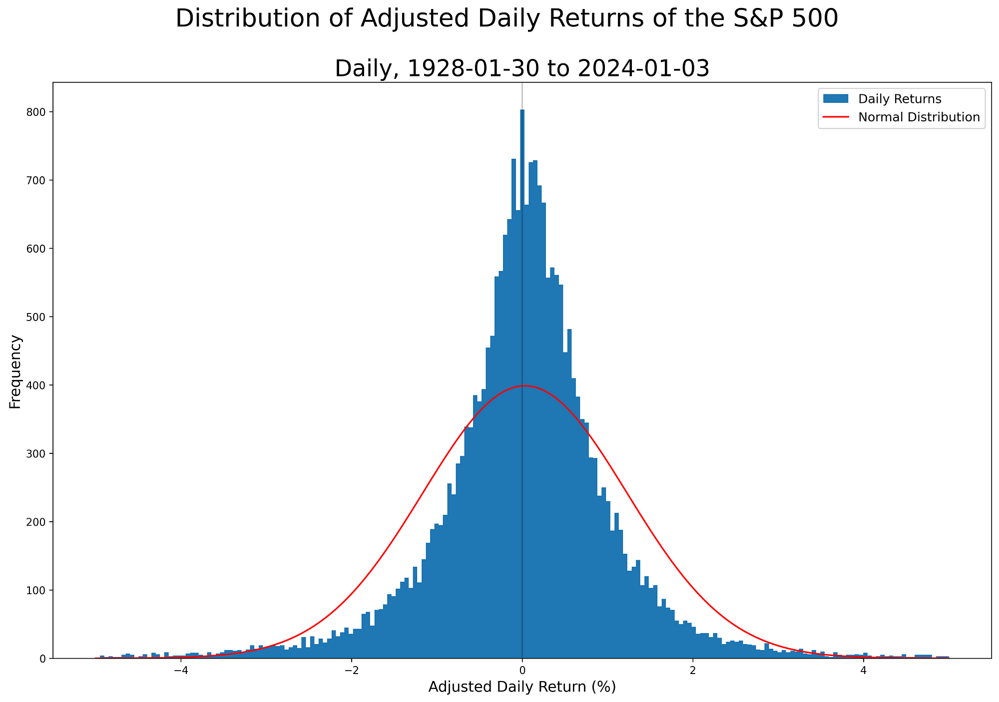
These characteristics of real return distributions are reflected in the shape of the volatility smile and smirk observed in options markets. The volatility smile shows implied volatilities that are higher for out-of-the-money and in-the-money options compared to at-the-money options, forming a U-shape when plotted against strike prices. The volatility smirk, more common in equity markets, shows higher implied volatilities for out-of-the-money put options compared to call options, reflecting the market's pricing of downside risk.

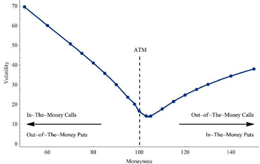
While the specific shape of real return distributions might not matter in a hypothetical frictionless and continuous market, real-world markets are neither frictionless nor continuous. This makes the actual distribution of returns highly relevant for risk management and option pricing. The major limitations to applying theoretical models directly are (1) models don’t adequately account for tail risk, which can be hedged using out-of-the-money options, (2) liquidity risk is a significant factor that's difficult to hedge effectively, (3) markets exhibit volatility clustering and regime changes, leading to volatility risk that can be addressed through volatility hedging strategies, (4) real markets have gaps, especially overnight and during weekends or market closures, which can only be partially mitigated through hedging.

The term structure of volatility can be partially attributed to these factors related to market frictions (the more real-world risks there are the more expensive the option). The resulting volatility surface, combining both strike and maturity dimensions, provides a more comprehensive view of how the market prices options across different strikes and expirations. This surface reflects the market's aggregate expectations of the effects of skew, kurtosis, and term structure.

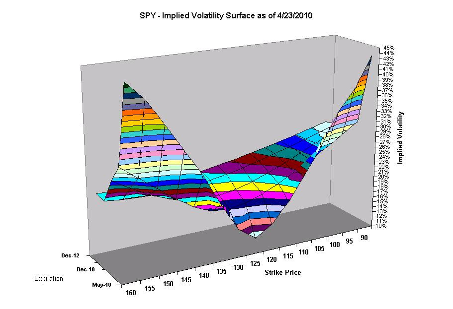
In the Black-Scholes world, implied volatility is constant across all strikes and time, but that is simply not the case in the real world. As such, this presents a difficult problem in defining the “true” implied volatility of returns. The development and widespread adoption of the VIX index is one of the most significant achievements in modern financial history for it allowed a way to capture the market's expectation of future volatility in a way that is largely model-agnostic.

VIX Construction

The original VIX construction method can be found in Robert Whaley’s “Derivatives on Market Volatility: Hedging Tools Long Overdue,” Journal of Derivatives, Fall 1993, page 71–84. Note that the VIX itself is just an index (i.e. a number) that cannot be directly traded; rather CBOE was considering listing VIX futures when arguments against the original methodology were raised. The summary below is from page 516-520 of the Natenberg:

The original VIX was calculated from calls and puts at the two exercise prices that bracketed the index price—essentially the at-the-money options. For a given expiration month, the call and put implied volatilities at each exercise price were averaged, and these were then weighted by the difference between the exercise price and the index price to yield an implied volatility for that expiration month. In order to determine a theoretical 30-day implied volatility, the two near-term expiration months were weighted to derive a final value.

When the exchange began planning for trading in VIX-related products, there were two major objections to the original calculation methodology. First, any exchange-traded product has to have a very well-defined value on which everyone can agree. If there are significant disagreements as to the value of a contract, especially at expiration, some traders will feel that they are being treated unfairly. This will certainly inhibit trading in the product and might, in some situations, lead to legal action against the exchange. The original VIX calculation required a theoretical pricing model to determine implied volatilities. This in itself can result in disagreements. Which model should be used? The Black-Scholes model? The binomial model? Some other more exotic model? (Recall from Chapter 22 that the OEX is an American option, carrying with it the right of early exercise.) Even if there is general agreement on an appropriate model, there may be disagreements as to the inputs into the model. What interest rate ought to be used? What dividend assumptions should be made? The exchange concluded that if it wanted to introduce trading in VIX related products, it would be necessary to improve on the existing calculation methodology.

The second objection had to do with the fact that only at-the-money options were used to calculate VIX values. As traders became more knowledgeable about options, the volatility skew, or smile, became increasingly important in describing the volatility environment and in determining appropriate strategies. Traders wanted an implied volatility index that would encompass not only the implied volatility of at-the-money options but also the implied volatility across a broad range of exercise prices.

The question we want to answer: “is it possible to create an option position that will capture the true volatility of the underlying contract under all possible volatility scenarios?” The answer to this question, assuming that the underlying follows some drift-diffusion process, is yes. The solution was first published by Kresimir Demeterfi, Emmanuel Derman, Michael Kamal, and Joseph Zou, in “More than You Ever Wanted to Know about Volatility Swaps,” Goldman Sachs Quantitative Strategies Research Notes, New York, March 1999.

The derivation for the construction method is a bit technical, and skipped in most textbooks. But I now offer a presentation of a heuristic, non-rigorous argument from stackexchange that I think should be understandable for readers who are comfortable with their background in calculus.

Let t0, t1, …, tn be observation times and St be the underlying price at time t. Then the realized variance of log returns, recalling 252 trading days a year, is defined as

\frac{252}{n}\sum_{i=1}^n \ln^2 \frac{S_{t_i}}{S_{t_{i-1}}}

Note that for sufficiently small x we have

\ln (1+x) \approx x - \frac{1}{2}x^2

\ln^2 (1+x) \approx x^2\approx 2x - 2 \ln(1+x)

Therefore, the realized log variance can be approximated

\begin{align*} \sum_{i=1}^n \ln^2 \frac{S_{t_i}}{S_{t_{i-1}}} &\approx 2\sum_{i=1}^n \frac{S_{t_{i}}-S_{t_{i-1}}}{S_{t_{i-1}}}-2\ln\frac{S_T}{S_0}. \end{align*}

Assuming that the interest rate 𝑟 is deterministic we can write

\begin{align*} E\bigg(\sum_{i=1}^n \ln^2 \frac{S_{t_i}}{S_{t_{i-1}}}\bigg) &\approx 2\sum_{i=1}^n E\Bigg(E\bigg(\frac{S_{t_{i}}-S_{t_{i-1}}}{S_{t_{i-1}}}\mid S_{t_{i-1}}\bigg)\Bigg)-2E\bigg(\ln\frac{S_T}{S_0}\bigg)\\ &= 2\sum_{i=1}^n E\Bigg(\frac{S_{t_{i-1}}e^{\int_{t_{i-1}}^{t_i}r_s ds}-S_{t_{i-1}}}{S_{t_{i-1}}}\Bigg)-2E\bigg(\ln\frac{S_T}{S_0}\bigg)\\ &= 2\sum_{i=1}^n \Big(e^{\int_{t_{i-1}}^{t_i}r_s ds} -1\Big)-2E\bigg(\ln\frac{S_T}{S_0}\bigg)\\ &\approx 2\sum_{i=1}^n \int_{t_{i-1}}^{t_i}r_s ds - 2E\bigg(\ln\frac{S_T}{S_0}\bigg)\\ &= 2\int_0^T r_s ds - 2E\bigg(\ln\frac{S_T}{S_0}\bigg)\\ &= 2\ln \Big(S_0 e^{\int_0^T r_s ds} \Big) - 2 \ln S_0 - 2E\bigg(\ln\frac{S_T}{S_0}\bigg)\\ &= -2E\bigg(\ln\frac{S_T}{E(S_T)} \bigg). \end{align*}

The second approximation is valid since for sufficiently small x

e^x-1 \approx x

Recall now the Integral Remainder form of Taylor’s Theorem, that for any smooth function f with positive a and x we have

\begin{align*} f(x) = f(a) + f'(a)(x-a) + \int_a^{\infty}(x-k)^+ f''(k)dk + \int_0^a (k-x)^+f''(k)dk. \end{align*}

If we substitute in f(x) = ln(x), x = S(T), and a = E(S(T)) then

\begin{align*} \ln S_T = \ln E(S_T) + \frac{S_T - E(S_T)}{E(S_T)} - \int_{E(S_T)}^{\infty} \frac{(S_T-k)^+}{k^2} dk - \int_0^{E(S_T)} \frac{(k-S_T)^+}{k^2} dk. \end{align*}

It follows immediately that

\begin{align*} E\bigg(\sum_{i=1}^n \ln^2 \frac{S_{t_i}}{S_{t_{i-1}}}\bigg) &\approx -2E\bigg(\ln\frac{S_T}{E(S_T)} \bigg)\\ &=2E\bigg[\int_{E(S_T)}^{\infty} \frac{(S_T-k)^+}{k^2} dk + \int_0^{E(S_T)} \frac{(k-S_T)^+}{k^2} dk\bigg], \end{align*}

which is a sum of the prices of puts ((k−S(T))+) and calls ((S(T)−k)+) weighted by the reciprocal of strike (k) squared. The above works for 1-year variance exposure, but how should we scale our exposure with time? Intuitively, we should weigh by the reciprocal of time (since variance is proportional to time under a diffusion model). We now confirm this; recalling that the log returns are dragged by half of variance

\begin{align*} S_T &= S_0 \exp\big((r-\frac{1}{2}\sigma^2)T+\sigma W_T \big)\\ &= E(S_T) \exp\big(-\frac{1}{2}\sigma^2T+\sigma W_T \big) \end{align*}

The variance is given by

\sigma^2 =\frac{2}{T}\Big(\sigma W_T -\ln \frac{S_T}{E(S_T)} \Big)=-\frac{2}{T}E\Big(\ln \frac{S_T}{E(S_T)}\Big)

Why do we have to weigh by the reciprocal of the strike squared (other than the math said so)? From the Natenberg:

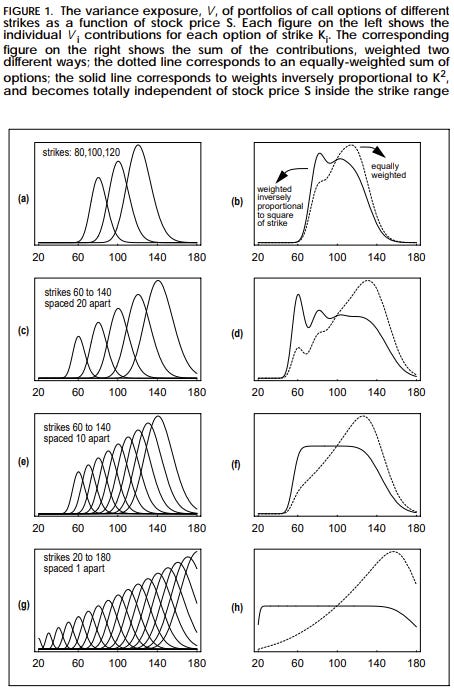
Perhaps the greatest drawback to [buying one option and delta hedging] is the fact that exposure to the volatility of the underlying market, as measured by the vega, will change over the life of the strategy. An option’s vega value is greatest when the option is at the money, but even if we begin by purchasing at-the-money options, the options will almost certainly not remain at the money. As the underlying price rises or falls, the options will either go into the money or out of the money, and the vega of the position will decline.

If we want to create a long volatility position, we want a constant exposure to volatility regardless of changes in the price of the underlying contract. We might try to accomplish this by purchasing options across a broad range of exercise prices. In this scenario, one exercise price will always be at the money. Unfortunately, this will still not result in a constant vega exposure because at-the-money options with higher exercise prices have greater vega values than at-the-money options with lower exercise prices. If we add up all the vega values at each underlying price, the total vega will be lower at lower underlying prices and higher at higher underlying prices.

Note that the problem here is that vega is defined as the sensitivity of option value to volatility, but volatility is defined in % terms to the price of the underlying. Imagine at-the-money options with different strikes but all else held equal, we should expect option prices to have higher exposure to volatility as strikes increases since at higher prices the same volatility implies a larger expected move in the underlying in $ terms.

The vega of options has a linear relationship with the strike, all else held equal (this is intuitive since the same vol implies larger moves at larger strikes, increasing in a linear fashion), and so the exposure of options to variance (instead of volatility) increases quadratically with strike, implying a weighting scheme that is proportional to the reciprocal of strike squared. Graph below is from the original Goldman paper; note that in figures (g) and (h) by placing options closely we are able to have a constant Vega exposure across a large range of strikes

Given this weighting scheme, the other steps of constructing the VIX becomes trivial. The complete methodology is 22 pages long and is given out by CBOE, but Natenberg page 520-521 gives a good summary.

Essentially, the value of the VIX is the cost of purchasing a strip consisting of options at every available exercise price [weighted inversely to the square of strike]. Because the VIX represents a 30-day implied volatility, the value of the VIX is derived from strips of options in the two monthly expirations that bracket 30 days. The values of the strips are then weighted by how close each expiration is to 30 days.

The value of the VIX is derived from the volatility value (time value) of the options in the underlying index, not the intrinsic value. Therefore, only the prices of out-of-the-money options (compared with the forward price) are used. The (implied) forward price for the index is determined using put-call parity for the closest-to-the-money exercise price. The option value used at each exercise price is the average of the quoted bid price and ask price.

When two exercise prices with a nonzero bid are encountered, no lower exercise prices for puts or higher exercise prices for calls are included in the calculation. Because only a finite number of exercise prices are available, the contribution of each option to the final VIX calculation is adjusted based on the distance between consecutive exercise prices. The greater the distance between exercise prices, the greater is the weighting in the index for a specific option.

Because the VIX represents a theoretical 30-day implied volatility, traded contracts on the VIX typically expire 30 days prior to expiration of the options used to calculate VIX values, usually the third Wednesday of the previous month. VIX January contracts expire 30 days prior to expiration of February SPX options; VIX February contracts expire 30 days prior to expiration of March SPX options; and so on.

Characteristics of VIX and Vol (From Colin Bennett)

The VIX is an index just like the SPX (S&P 500) index, and therefore traders can gain exposure to the VIX though trading VIX futures, just like they can gain exposure to the S&P 500 by trading SPX futures. In both cases, no option or stock need to exchange hands, a futures contract is simply opened and both sides post margin per instructions by the clearinghouse as the futures price changes. We now explore some of the characteristics of volatility products which will lead to an understanding of why so many piled onto the short vol trade, and how it blew up so spectacularly. I quote directly from Colin Bennett most of the points below.

(1) The apparent “overpricing” of volatility (Implied Vol > Realized Vol) is misleading. Selling implied volatility is one of the most popular trading strategies in equity derivatives, but the mere fact that implied vol is often greater than realized vol does not necessarily mean that the strategy is profitable.

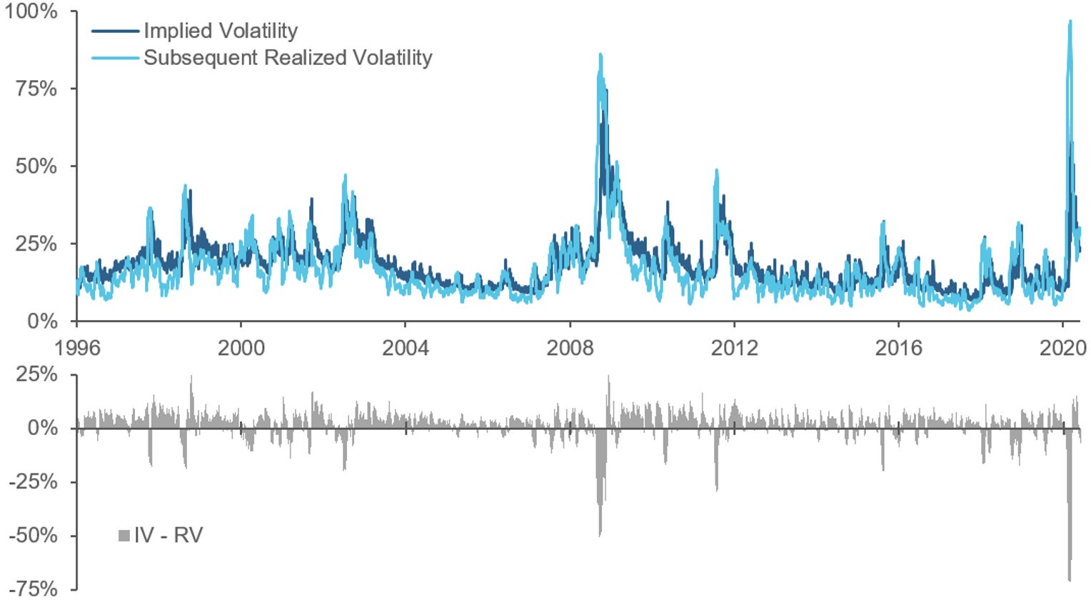
This is since when realized vol spikes, it typically goes significantly above implied vol. In addition, it is impossible to gain direct exposure to volatility using put and calls since they are exposure to the variance, not the volatility, of returns. As such, during vol spikes, the losses from shorting vol is quadratic instead of linear.

(2) However, as volatility is negatively correlated to equity returns, a short volatility (or variance) position is implicitly long equity risk. As equity returns are expected to return an equity risk premium over the risk-free rate, this implies short volatility should also be profitable. Fundamentally, vol and equity should be negatively correlated because lower equity prices increase corporate leverage, and holding enterprise vol constant, increased leverage increases equity vol.

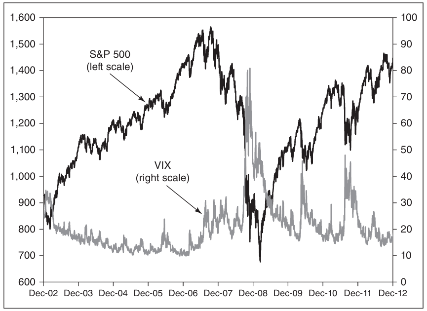
Note that the % change in the VIX is approximately 5x-6x times greater than the % change in the S&P 500, but in the opposite direction.

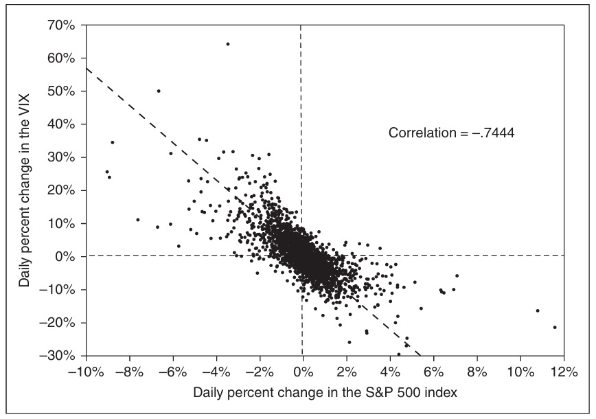
However, it is worthy to note that realized vol is less negatively correlated with equity returns when compared to implied vol; there is a moderate inverse correlation of –0.4 instead of the -0.75 for implied vol. Perhaps the effect of equity drawdowns on the VIX is a combination of both heightened volatility and heightened demand for put protection (it noteworthy that VIX returns and subsequent realized vol changes have negligible correlation).

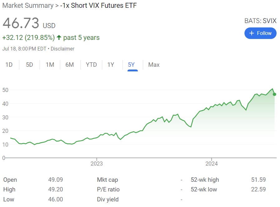
(3) There are several fundamental reasons why volatility may have been overpriced in addition to equity risk premium (the rise in AUM of short vol funds and covered call funds may have changed this dynamic today). Demand for put protection and demand for hedging products, either from investors, structured products or providers of variable annuity products, needs to be offset by market makers. As market makers are usually net sellers of volatility, they charge margin for taking this risk and for the costs of hedging. Below are returns from the SVIX ETF that shorts VIX futures

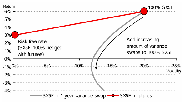
(4) Long vol is a poor equity hedge. An ideal hedging instrument for a security is an instrument with -100% correlation to that security and zero cost. The return on variance swaps have a c-70% correlation with equity markets, but they are also on average overpriced so we may suspect that the cost of this strategy far outweighs any diversification benefit. Below are returns from the VIXY ETF that longs VIX futures

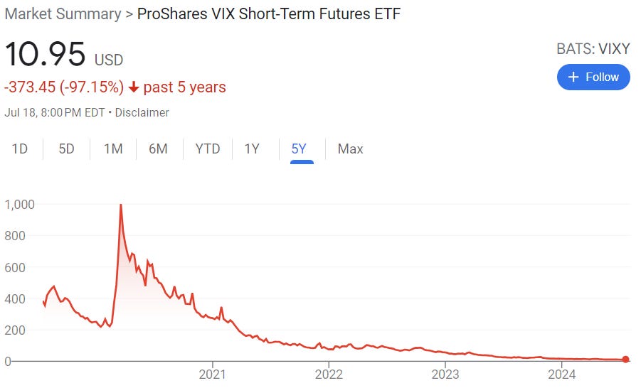
Note that long volatility should have below market returns for three reasons: (1) that it is short equity risk premium and that (2) vol itself is overpriced due to demand for insurance on market portfolios (the world by definition is net long the market) (3) vol is itself highly volatile and so the vol of vol creates a drag on the compounded annual growth rate for any strategy that attempts to maintain a fixed exposure to vol. If any investor wants to hedge equity risk, there is no reason why they cant just short futures and therefore reduce net equity exposure. This is consistent with CAPM.

(5) VIX futures curve typically trades in contango (upward sloping) due to the interplay between short-term and long-term volatility expectations, hedging dynamics, and the nature of volatility itself. In the short term, VIX futures are often closely tied to realized volatility because traders can effectively replicate and hedge these positions through dynamic hedging. This hedging activity creates a strong link between short-term futures and current market conditions, effectively "pinning" them closer to realized volatility levels. The lower risk associated with shorter time horizons also contributes to this phenomenon, as there's less uncertainty about potential market moves in the immediate future.

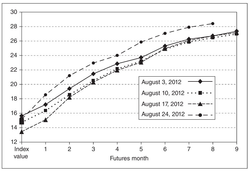
For longer-term VIX futures, however, implied volatility tends to be higher, reflecting increased uncertainty and risk over extended periods. This upward slope in the term structure mirrors the volatility smile observed in options markets, where out-of-the-money options (especially puts) often have higher implied volatilities. The potential for large, unexpected market moves over longer time frames raises both the wings of the volatility smile and the long end of the VIX term structure.

(6) During periods of market stress or heightened uncertainty, the VIX term structure can shift into backwardation, where near-term VIX futures trade at higher levels than longer-dated contracts. The near-month VIX futures contracts tend to move more dramatically than far-month contracts during these events; this disproportionate movement in the front end of the curve is rooted in the nature of volatility itself – volatility tends to cluster and exhibit strong autocorrelation, but is also mean-reverting and stationary.

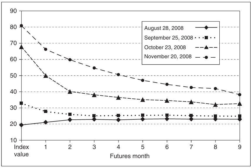
This phenomenon is observed not only in implied volatility but also in realized volatility, where short-term realized volatility can fluctuate wildly while long-term realized volatility remains relatively stable.

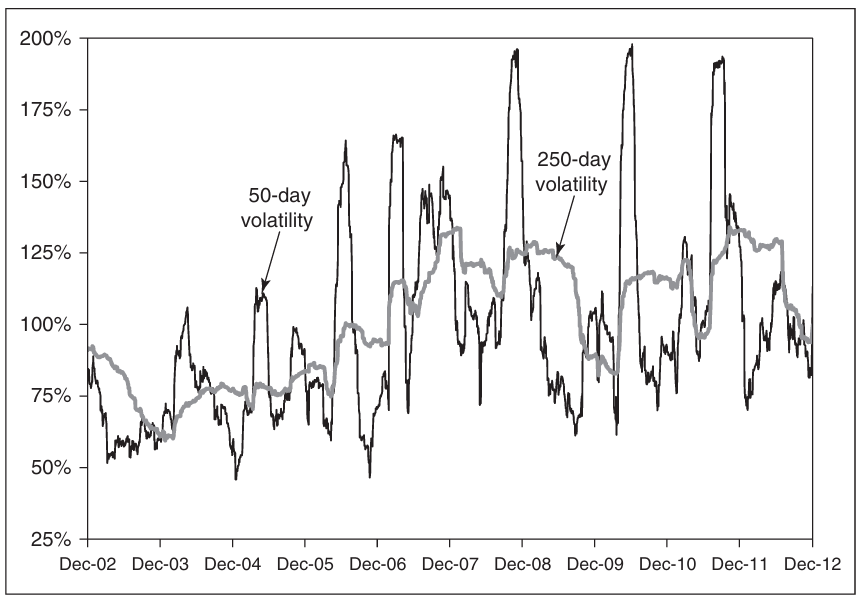
In fact, there is correlation between volatility term structure and volatility skew that arises from the similar dynamics that govern them. Both long-term implied volatility and the implied volatility of far out-of-the-money options are relatively "pinned" or stable compared to their short-term or at-the-money counterparts. For instance, a sudden 10% drop in the S&P 500 over a week, while significant, doesn't substantially increase the probability of a further 50% decline, nor does it dramatically alter the expected volatility two years into the future.

Volmageddon

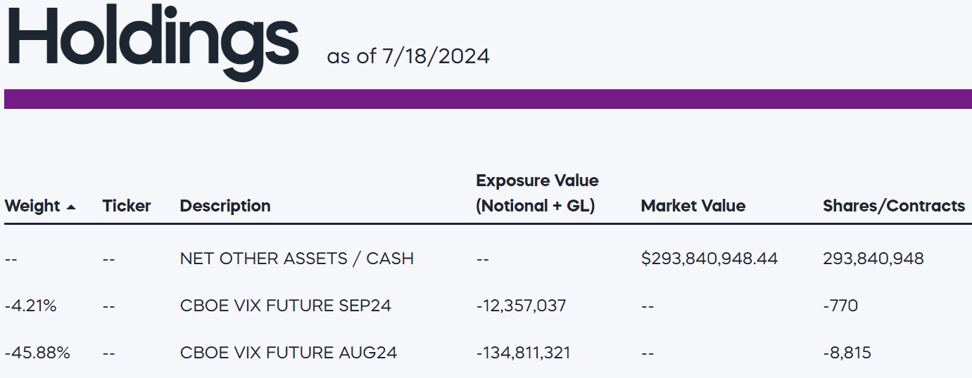
The properties of VIX futures listed above suggest that shorting them may be an attractive preposition. Indeed, that is what ETFs such as $SVXY (ProShares Short VIX Short-Term Futures ETF). The fund’s holdings are available publicly, and as expected, it holds short positions in VIX futures in addition to holding cash. During trading hours, it needs to actively buy / sell futures in order to maintain its target exposure (in this case, -0.5). You can find its factsheet here.

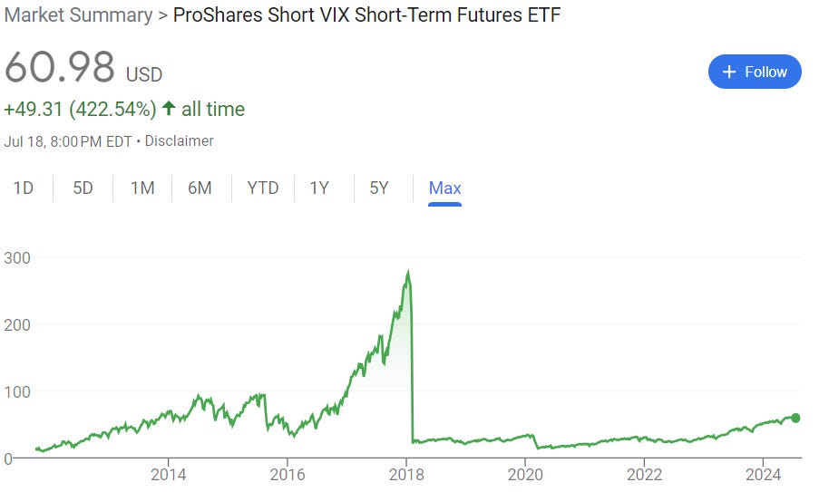
While the returns of short VIX funds have been pretty good in the from the post COVID recovery to now, they were nothing compared to the returns generated prior to February 5 2018. How good were these returns? SVXY returned more than 650% in the two years immediately prior (and has yet to recover, partially because it has been deleveraged from -1x to -0.5x VIX futures).

There are a few structural features about Exchange-Traded Products that we now note. (1) First, issuers have wide discretion over the management of their funds. While they do have a fiduciary responsibility to target their index with whatever leverage the fund advertises, they are also able to deviate from that mandate if it is clear that it is in the best interest of their shareholders to do so. For example, when oil prices went negative in front month futures, managers for USO switched to other months in order to save the fund. ETP issuers must maintain the ability to terminate their funds in the event of extreme intraday market movements to prevent the fund's value from becoming negative, though this protective measure can disadvantage shareholders by eliminating potential benefits from subsequent market reversals.

(2) The daily rebalancing process of these ETPs can amplify market trends, as both leveraged long and inverse funds are compelled to adjust their VIX futures positions in ways that reinforce prevailing market directions. During volatility spikes, for instance, inverse funds must reduce leverage by covering short positions, while leveraged long funds increase exposure by acquiring additional VIX futures or equivalents, both requiring them to buy more volatility contracts.

(3) ETP issuers often utilize over-the-counter swap agreements to outsource this rebalancing process to institutional counterparties, transactions that lack transparency to external observers. These counterparties typically hedge their risk exposure through VIX futures or analogous strategies, such as delta-hedged S&P 500 index (SPX) straddles. These mechanisms, while necessary for the operation of volatility ETPs, can have significant implications for market dynamics, particularly during periods of heightened volatility.

By January 2018, partially as the result of the spectacular returns that they have generated, (4) the combined assets of inverse and leveraged volatility funds had grown to over $5 billion. Note that the internal position adjustments required for these funds' end-of-day resets are proportional to both their asset size and the daily percentage move of the volatility index. With $5 billion in total assets, a mere 10% move could trigger a combined buying need of $500 million worth of futures. These figures were substantial relative to the overall VIX futures market, which had a notional value of only around $7-$10 billion typically at the time, meaning the rebalancing needs of a single ETP could represent a significant portion of the market.

It should also be noted (5) that the covering of short vega (i.e. short volatility) positions by buying vega may actually increase the short vega position through a combination of market impact and vega convexity. To elaborate, recall that the derivative of vega with respect to vol, also called vomma, is positive everywhere.

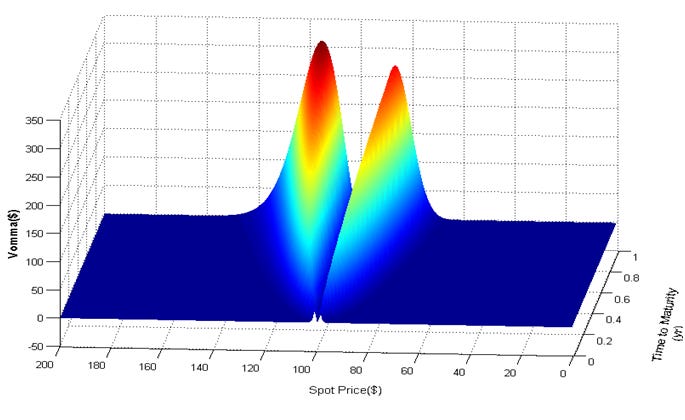
For a single call option, vomma is almost 0 near the money but expands towards the wings. However, recall that the VIX is replicated by a chain of options, as such its Vomma exposure, like its vega exposure, is roughly equal everywhere. As such, when the vega of options increases with rising volatility the short volatility position is enlarged and necessitates more hedging. This creates a self-reinforcing cycle of volatility buying and increasing implied volatility, which necessitates more buying.

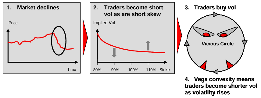
Conversely, during market recoveries, funds become long volatility and must sell, potentially causing implied volatility to undershoot. This mechanism elucidates why implied volatility often appears to react more extremely than warranted by market movements alone, highlighting the significant impact of structured products and large financial institutions' hedging activities on market dynamics, particularly during periods of stress or rapid recovery.

February 5th 2018 did indeed start with a market sell off. Not much really happened that day, but yields ticked up and stocks sold off as investors worried about inflation caused by a strong job market. Stocks sank throughout the day, then went off a cliff in the final hour of trading. The Dow was down 800 points at 3 p.m. but within minutes, it was down 1,500 points (The only reason I am using the Dow is because CNN has a good graphic for it, the S&P 500 was roughly down 4%).

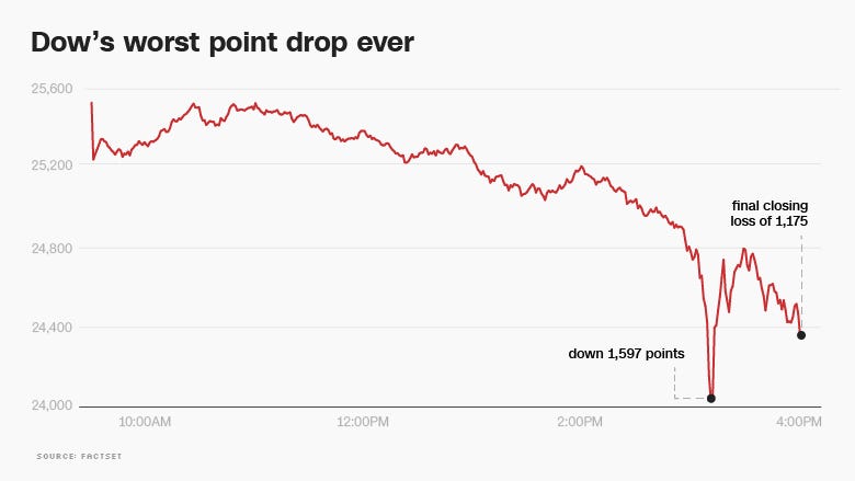
The sharp drop in the market was at an extreme inopportune timing, less than an hour before VIX futures settlement, vol was up 20% with signs of market panic. Barring a reversal, this situation implied a minimum of $800 million worth of VIX futures would need to be purchased by ETPs or their counterparties at the 4:15 PM ET futures market close. This impending demand was apparent to market participants, likely prompting traders to acquire VIX futures in anticipation of a price surge, while existing futures holders were disinclined to sell. The confluence of these factors set the stage for a potential price run-up near the final settlement time, highlighting the systemic risks posed by the growing influence of volatility ETPs on the broader VIX futures market.

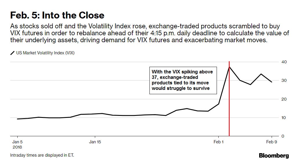
The rest is history. The buying activity that ensured resulted in the largest VIX move in both percentage (+116%) and point moves (+20) since the VIX's inception in 1993 (this was disproportionate to the coincident 4.1% drop in the S&P 500, which ranked only 31st in magnitude over the same period).

The VIX spike's culminated in a catastrophic liquidity event on the afternoon of February 5th, 2018. Exchange Traded Fund managers and counterparties tracking indexes needed to acquire approximately $4 billion worth of VIX futures or equivalent volatility instruments at the ~4:15 PM ET futures close (assuming they followed their mandates). The fact that the market had not experienced a one-day downswing of this magnitude in nearly two and a half years probably did not help. The most recent previous comparable event occurring on August 15, 2015 (-3.96%). The extended period of low volatility had probably fostered complacency among traders and fund managers. Faced with this unprecedented buying pressure, VIX futures liquidity evaporated, causing futures prices to soar in the final minutes of trading.

Some fund managers, notably ProShares (managing SVXY and UVXY), either chose not to complete their purchases or were unable to fill their orders on February 5th. This inaction, while risky if volatility had continued to spike, ultimately benefited their shareholders as volatility decreased on February 6th.

Credit Suisse announced the termination of XIV on February 6th, with February 15th set as its last trading day. The -97% move on February 5th triggered the "acceleration event" clause in their prospectus, allowing for fund shutdown if daily losses met or exceeded 80%. By the end of February 2018, both ProShares, reportedly under SEC pressure, reduced the leverage on their volatility funds to mitigate the risk of similar future drawdowns. While lawsuits were filed and accusations made, no definitive judgments had been handed down to my knowledge.

The event dispelled the notion that VIX futures are inherently less volatile than the VIX itself, introducing a more realistic understanding of these instruments' risks. As of February 2019, assets in short-term leveraged/inverse volatility products had decreased to approximately $1 billion, a significant reduction from $5 billion.

This reduction in asset values substantially lowered the risk of a similar event recurring. The Volmageddon event served as a stark reminder of the potential risks associated with complex volatility products and led to a more cautious approach in the market. The reduction in assets under management in these products, combined with increased awareness of their risks, has potentially created a more stable environment. However, it remains crucial for investors and regulators to continue to assess the systemic risks posed by complex financial instruments.

VIX Contract Applications

The case study of Volmageddon make VIX products look like tools of pure speculation. However, real, economically productive uses for VIX futures do exist. To quote from Natenberg pages 537-538:

Hedge fund managers sometimes acquire volatility positions, perhaps unintentionally, as a result of their market activities. If they want to hedge away some of this volatility risk, variance and VIX contracts offer a simple way of doing this. A trader who has a realized volatility position, either a positive or negative gamma, can trade variance contracts to hedge his realized volatility risk. A trader who has an implied volatility position, either a positive or negative vega, can trade VIX contracts to hedge his implied volatility risk.

An option market maker typically profits from higher option trading volume. But higher volume is often the result of higher volatility. When there is greater volatility, there is greater demand for options. As such, the market maker has an indirect long volatility position…To hedge this indirect long volatility position, market makers sometimes take a short volatility position in volatility contracts, most commonly the VIX. Of course, the market maker is really hedging trading volume.

Another type of indirect volatility position is one in which a portfolio manager is required to periodically rebalance a portfolio. There is a cost to the rebalancing process, and the cost is typically higher in times of high volatility when bid-ask spreads tend to widen. The portfolio manager therefore takes on a short volatility position as the rebalancing period approaches. He can hedge this short volatility position by taking a long volatility position in the VIX.

Finally, and perhaps most importantly, we note that VIX futures facilitate efficient risk transfer between different types of market participants. When traders short VIX futures in anticipation of profit, they effectively lower the price of put options used for portfolio protection. This mechanism creates a risk transfer channel where less risk-averse participants (those shorting VIX futures) take on risk from more risk-averse participants (those seeking portfolio protection through put options). This process is intermediated by options market makers, who balance supply and demand in the options market. While the overall transaction may be zero-sum in terms of financial gains and losses, it generates positive utility for the market as a whole. It allows for a more efficient allocation of risk, with risk-tolerant investors absorbing volatility risk from those who are less willing or able to bear it.